from Chapter8code import *9 Distributed Plasticity
In earthquake engineering, concentrated plasticity elements were common when nonlinear analysis emerged as a viable tool. However, in nonlinear dynamic analysis, concentrated plasticity can cause large spurious forces, depending on the prescribed damping model. The distributed plasticity element presented in this chapter alleviates that problem. Another advantage of the element presented here is the high granularity in the modelling of yielding and thus damage from cyclic loading. It is also a plus that a variety of cross-section and material models can be used as part of this element.
As illustrated in Figure 9.1, the distributed plasticity element contains cross-sections, which in turn contain uniaxial hysteretic materials. This discretization is related to numerical integration for element and cross-section integrals that appear later in this chapter. The element has one cross-section instance at each integration point. Similarly, the uniaxial materials are the integration points of the cross-section. These uniaxial models are referred to as fibres.
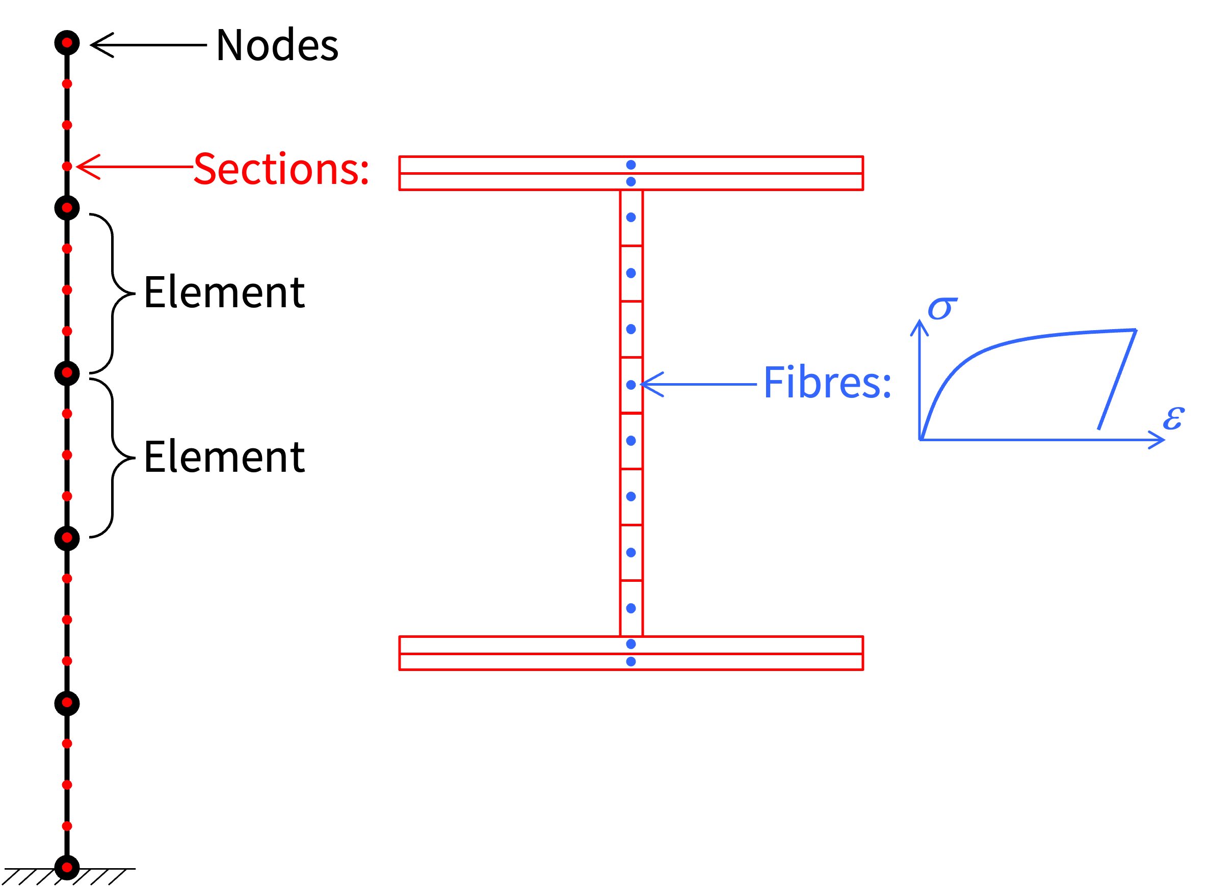
The specific element, cross-section, and material models employed in this chapter are
- Displacement-based distributed plasticity element (presented in this chapter)
- Wide-flange cross-section (presented in this chapter)
- Bilinear hysteretic material (presented in the previous chapter)
Two formulations are available for distributed plasticity frame elements:
- The “displacement-based” formulation employs shape functions known from introductory courses on the finite element method, i.e., interpolation of displacement between the DOFs of the element. This formulation is pedagogical, and is pursued in this chapter, but limits how curvature varies along the element. Columns in a real building shook by strong ground motion tend to exhibit concentrated curvature. In this book, this is referred to as Element 12.
- The “force-based” formulation for distributed plasticity elements does not limit the variation of curvature along the element, meaning one element may be sufficient along the full height of a column member. Instead of displacement interpolation, this element is based on interpolating the bending moment along the element from force values along the DOFs of the element. This is labelled Element 13 in this book. The state determination, and the associated response sensitivity calculations, are somewhat more cumbersome for this element compared with Element 12.
The hierarchy of elements, cross-sections, and fibres outlined in Figure 9.1 means that the state determination needs to send trial displacements from the Newton-Raphson algorithm through the elements, through its cross-sections, ultimately received as trial strain by the hysteretic uniaxial material model in each fibre. That process is illustrated in the right-hand side of Figure 9.2. This figure is valid for Element 12, i.e., the displacement-based distributed plasticity element. DOF configurations and transformation matrices introduced in Chapter 3 appear here as well, but two new “levels” are introduced at the bottom of Figure 9.2. Specifically, a Section has two DOFs: axial and moment. That means \(\mathbf{u}_s=\{\varepsilon, \; \kappa\}\), where \(\kappa=\) curvature and \(\mathbf{F}_s=\{N, \; M\}\), where \(N=\) axial force and \(M=\) bending moment.
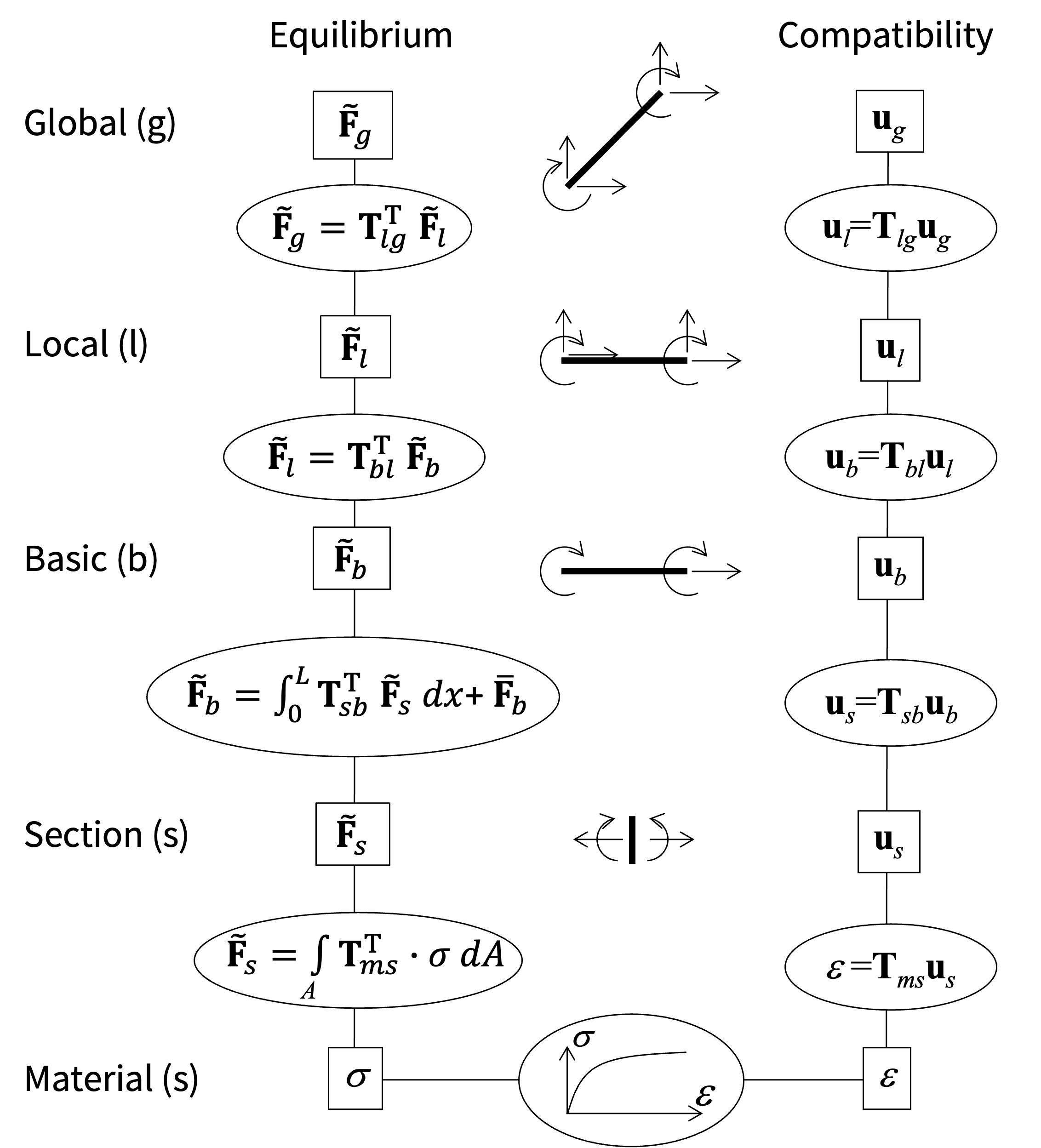
Still with reference to Figure 9.2, the transformation between the Material and Section level is straightforward beam theory. The transformation “matrix” \(\mathbf{T}_{ms}=\{1, \; -z\}\) expresses that \(\varepsilon(z) = \varepsilon_{\mathrm{axial}} - z \cdot \kappa\), where \(z=\) upwards distance from the centroid of cross-section to the fibre, and tension is positive.
The transformation between the Section and the Basic element requires the concept of shape functions from finite element analysis. A shape function expresses the displaced anywhere in the element due to a unit displacement at the DOF associated with the shape function. Using the Basic DOF numbering from Figure 3.1, here is a plot of the respective shape functions, using a unit element length for this demonstration:
L = 1
x = np.linspace(0, L, 100)
N1 = x/L
N2 = -1/L**2 * x**3 + 2/L*x**2 - x
N3 = -1/L**2 * x**3 + 1/L*x**2
fig, axs = plt.subplots(3)
axs[0].plot(x, N1, 'k-')
axs[1].plot(x, N2, 'k-')
axs[2].plot(x, N3, 'k-')
plt.show()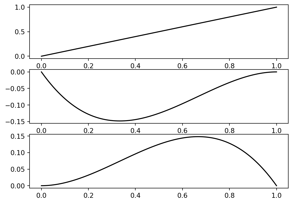
Looking at those graphs, we recognize at the top a linear increase in axial displacement from zero on the left-hand side to unity on the right-hand side. That is a proper shape function because it gives the amount of axial displacement along the element due to a unit value of the corresponding axial DOF. In the bottom graphs shown above we see the displaced shape due to a unit rotation of the second and third Basic DOF, i.e., the clockwise rotation on the left- and right-hand side of the element.
To determine \(\mathbf{T}_{sb}\) we acknowledge that it is defined by the relationship \(\mathbf{u}_s = \mathbf{F}_{sb} \mathbf{u}_b\), with \(\mathbf{u}_s=\{\varepsilon, \; \kappa\}\) defined above and \(\mathbf{u}_s=\{u_{b1}, \;u_{b2}, \;u_{b3}\}\). Beam theory says that \(\varepsilon = \frac{du}{dx}\) and \(\kappa = \frac{d^2w}{dx^2}\), where \(w=\) transversal displacement, i.e., displacement in the \(z\)-direction, examplified in the bottom two graphs below Listing 9.1. That means the transformation matrix is obtained by differentiation of the shape functions:
\[ \begin{aligned} \begin{Bmatrix} \varepsilon \\ \kappa \end{Bmatrix} &= \underbrace{\begin{bmatrix} \frac{dN_1(x)}{dx} & 0 & 0 \\ 0 & \frac{d^2N_2(x}{dx^2} & \frac{d^2N_3(x}{dx^2} \end{bmatrix}}_{\mathbf{T}_{sb}} \begin{Bmatrix} u_{B1} \\ u_{B2} \\ u_{B3} \end{Bmatrix} \\ &= \underbrace{\begin{bmatrix} \frac{1}{L} & 0 & 0 \\ 0 & \left( -\frac{6x}{L^2} + \frac{4}{L} \right) & \left( - \frac{6x}{L^2} + \frac{2}{L} \right) \end{bmatrix}}_{\mathbf{T}_{sb}} \begin{Bmatrix} u_{B1} \\ u_{B2} \\ u_{B3} \end{Bmatrix} \end{aligned} \tag{9.1}\]
where the notation \(N_i\) for the shape functions must not be confused with the symbol \(N\) for axial force. The two curvature components of \(\mathbf{T}_{sb}\) are visualized here:
kappa1 = -6*x/L**2 + 4/L
kappa2 = -6*x/L**2 + 2/L
fig, axs = plt.subplots(2)
axs[0].plot(x, kappa1, 'k-')
axs[0].axhline(0, color='black', linestyle='--', linewidth=1)
axs[1].plot(x, kappa2, 'k-')
axs[1].axhline(0, color='black', linestyle='--', linewidth=1)
plt.show()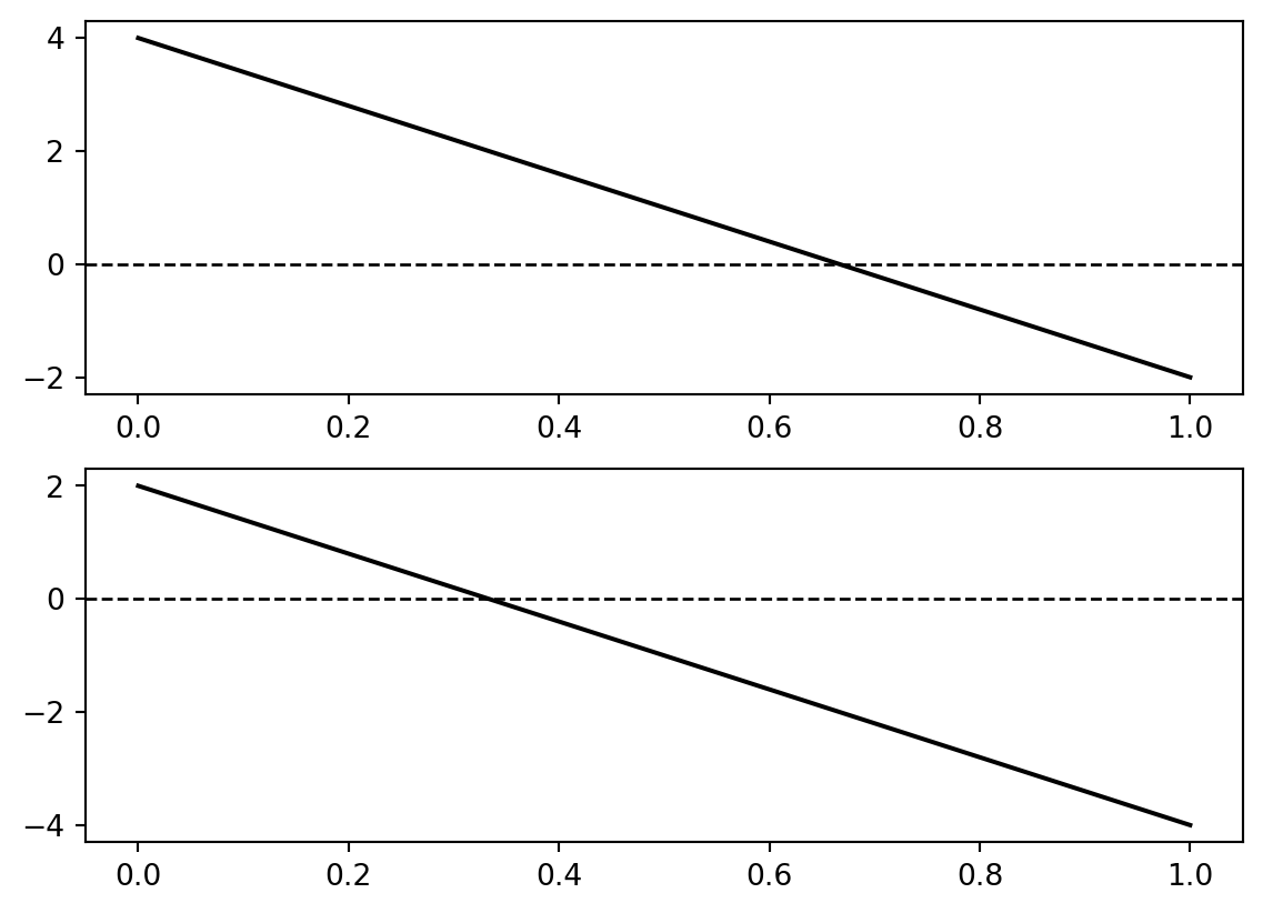
That plot confirms the linear variation in curvature along the element, a characteristic of the displacement-based distributed plasticity element. This is why several elements are needed along the length of a member who is undergoing damage, in order to capture concentrated curvature near the member ends.
9.1 Wide-flange Cross-section
The cross-section visualized in Figure 9.1 is implemented in this book. It has six input variables:
hw= \(h_w\) = total web heightbf= \(b_f\) = width of both flangestf= \(t_f\) = flange thicknesstw= \(t_w\) = web thicknessnf= \(n_f\) = number of fibres in each flangenw= \(n_w\) = number of fibres in the web
Only first-order sensitivities are here considered, which means that the following member functions of the cross-section class are implemented:
def __init__()(Constructor)def stateDetermination()def stateDerivative()def commit()def commitSensitivity()
Similar to the bilinear material in the previous chapter, the complete code is too large for a pedagogical presentation here. Instead, that code is made available in Appendix B and imported here:
from AppendixBcode import *It is instructive to examine the state determination from that imported code, as it was in the previous chapter for the bilinear material:
def stateDetermination(self, us):
    Ks = np.zeros((2, 2))
    Fs = np.zeros(2)
    for i in range(self.numfib):
        fiber = self.fibers[i]
        area = self.areas[i]
        loc = self.locations[i]
        Tms = np.array([-loc, 1])
        epsilon = Tms.dot(us)
        sigma, E = fiber.stateDetermination(epsilon)
        Ks = Ks + np.outer(Tms, Tms) * area * E
        Fs = Fs + Tms * area * sigma
    return Fs, Ks
In this implementation the rotational DOF is first and the axial DOF second because of legacy code, and \(z\) is called loc, but the compatibility and equilibrium equations from the bottom of Figure 9.2 are easily identified. The statement epsilon = Tms.dot(us) represents compatibility, and that strain is sent to the material model in the next line. Thereafter, the cross-section integral in Figure 9.2 sums force and stiffness contributions from all fibres of the cross-section.
An important point for the complete code in Appendix B relates to sensitivity analysis. The right-most term in Equation 8.10 requires the derivative of the internal forces for fixed current displacements. Interestingly, that does not mean for fixed current strain in the material. To understand that, suppose the web height, \(h_w\), is the variable \(x\) for which differentiation is carried out. A change in \(h_w\) implies a change in the fibre locations, represented by loc in Listing 9.3. In turn, that means \(\frac{\partial \mathbf{T}_{ms}}{\partial x}\) is non-zero. The consequence of that will be seen shortly, after first differentiating the last line in Listing 9.3 using the product rule of differentiation:
\[ \left. \frac{\partial \tilde{\mathbf{F}}_s}{\partial x} \right|_{\mathbf{u}_s \: \mathrm{fixed}} = \frac{\partial \mathbf{T}_{ms}^{\top}}{\partial x} \cdot A \cdot \sigma(\varepsilon) + \mathbf{T}_{ms}^{\top} \cdot \frac{\partial A}{\partial x} \cdot \sigma(\varepsilon) + \mathbf{T}_{ms}^{\top} \cdot A \cdot \left. \frac{\partial \sigma(\varepsilon)}{\partial x} \right|_{\mathbf{u}_s \: \mathrm{fixed}} \tag{9.2}\]
The conditional derivative in the last term is further expanded by the chain rule:
\[ \begin{aligned} \left. \frac{\partial \sigma(\varepsilon)}{\partial x} \right|_{\mathbf{u}_s \: \mathrm{fixed}} &= \frac{\partial \sigma(\varepsilon)}{\partial \varepsilon} \left. \frac{\partial \varepsilon}{\partial x} \right|_{\mathbf{u}_s \: \mathrm{fixed}} + \left. \frac{\partial \sigma(\varepsilon)}{\partial x} \right|_{\varepsilon \: \mathrm{fixed}} \\ &= E \cdot \frac{\partial \mathbf{T}_{ms}^{\top}}{\partial x} \mathbf{u}_s + \left. \frac{\partial \sigma(\varepsilon)}{\partial x} \right|_{\varepsilon \: \mathrm{fixed}} \end{aligned} \tag{9.3}\]
where the compatibility equation \(\varepsilon = \mathbf{T}_{ms}^{\top} \mathbf{u}_s\) is differentiated in the second factor of the first term on the right-hand side. In conclusion, \(\left. \frac{\partial \varepsilon}{\partial x} \right|_{\mathbf{u}_s \: \mathrm{fixed}}\) is not zero as might have been expected. This is correctly implemented in the functions stateDerivative() and commitSensitivity() in Appendix B.
9.2 Element Implementation
The equilibrium side of Figure 9.2 contains two integrals. The cross-section integral is addressed above, in Listing 9.3, with a loop over the fibres of the cross-section. The other integral in Figure 9.2 represents the “element integration” from \(0\) to \(L\), where \(L=\) element length. Readers familiar with the finite element method will know that Gauss quadrature, i.e., numerical integration is utilized for this purpose. The input nIP to the following function specifies the number of integration points:
def Gauss(nIP):
    if nIP == 2:
        xIP = [-.57735026918963, .57735026918963]
        weight = [1., 1.]
    elif nIP == 3:
        xIP = [-0.77459666924148, 0.0, 0.77459666924148]
        weight = [.55555555556, .88888888889, .55555555556]
    elif nIP == 4:
        xIP = [-.8611363116, -.3399810436, .3399810436, .8611363116]
        weight = [.3478548451, .6521451549, .6521451549, .3478548451]
    elif nIP == 5:
        xIP = [-.9061798459, -.5384693101, 0.0, .5384693101, .9061798459]
        weight = [.236926885, .4786286705, .5688888889, .4786286705, .236926885]
    elif nIP == 6:
        xIP = [-.9324695142, -.6612093865, -.2386191861, .2386191861, .6612093865, .9324695142]
        weight = [.1713244924, .3607615730, .4679139346, .4679139346, .3607615730, .1713244924]
    elif nIP == 7:
        xIP = [-.9491079123, -.7415311856, -.4058451514, 0., .4058451514, .7415311856, .9491079123]
        weight = [.1294849662, .2797053915, .3818300505, .4179591837, .3818300505, .2797053915, .1294849662]
    return xIP, weight
The constructor of Element 12 is shown here, essentially creating a wide-flange cross-section at every integration point:
class element12():
    def __init__(self, nsec, q, section, material, elno):
        self.q = q
        self.nsec = nsec
        sections = []
        for i in range(self.nsec):
            hw = section[1]
            bf = section[2]
            tf = section[3]
            tw = section[4]
            nf = section[5]
            nw = section[6]
            sec = wfsection(hw, bf, tf, tw, nf, nw, material)
            sections.append(sec)
        self.xip, self.weight = Gauss(self.nsec)
        self.no = elno
        self.secs = sections
Same as for Element 2, presented in Chapter 3, the transformation matrix \(\mathbf{T}_{bg}\) is set as a data member of the class when the initialize() function of the element is called. Notice in the implementation below the exception that counterclockwise rotation is positive and Basic the axial DOF is last because of legacy code:
class element12(element12):
    def initialize(self, xyz):
        dx = xyz[1,:] - xyz[0,:]
        self.L = np.sqrt(dx.dot(dx))
        self.dx = dx / self.L
        self.Tbg = np.array([[-self.dx[1]/self.L, self.dx[0]/self.L, 1.0, self.dx[1]/self.L, -self.dx[0]/self.L, 0.0],
                             [-self.dx[1]/self.L, self.dx[0]/self.L, 0.0, self.dx[1]/self.L, -self.dx[0]/self.L, 1.0],
                             [-self.dx[0],       -self.dx[1],        0.0, self.dx[0],         self.dx[1],        0.0]])
9.2.1 State Determination
The state determination visualized in Figure 9.2 means “walking down” the right-hand side of the figure, employing kinematic compatibility equations, followed by “walking up” the left-hand side, employing equilibrium equations. Those walks are implemented in the function shown below, where again the exception is made that counterclockwise rotation is positive and Basic the axial DOF is last, because of legacy code:
class element12(element12):
    def stateDetermination(self, xyz, ug, theLambda):
        ub = self.Tbg.dot(ug)
        points = self.xip
        weights = self.weight
        Fb = np.zeros(3)
        Kb = np.zeros((3, 3))
        for i in range(self.nsec):
            x = (points[i] + 1.0) / 2.0
            Tsb1 = (6.0 * x - 4.0) / self.L
            Tsb2 = (6.0 * x - 2.0) / self.L
            Tsb3 = 1.0 / self.L
            section = self.secs[i]
            Tsb = np.array([[Tsb1, Tsb2, 0.0],
                            [0.0,  0.0, Tsb3]])
            us = Tsb.dot(ub)
            Fs, Ks = section.stateDetermination(us)
            jacDet = self.L / 2
            Kb = Kb + np.einsum('ji,jk,kl->il', Tsb, Ks, Tsb) * (weights[i] * jacDet)
            Fb = Fb + np.transpose(Tsb).dot(Fs) * (weights[i] * jacDet)
        q = theLambda * self.q
        mom = q * self.L**2 / 12.0
        barFb = [mom, -mom, 0.0]
        Fb = Fb + barFb
        shear = q*self.L/2.0
        Fg = (np.transpose(self.Tbg)).dot(Fb) + np.array([-self.dx[1]*shear, self.dx[0]*shear, 0.0, -self.dx[1]*shear, self.dx[0]*shear, 0.0])
        Kg = np.einsum('ji,jk,kl->il', self.Tbg, Kb, self.Tbg)
        return Fg, Kg
Notice that the code above is essentially carrying out the element integral in Figure 9.2, looping over the integration points along the element.
9.2.2 First-order Sensitivities
Response sensitivities are obtained by differentiating the state determination presented above, which yields:
class element12(element12):
    def stateDerivative(self, xyz, ug, theLambda, ddmParameter, ddmIndex, ddmIsHere, dKflag='none'):
        ub = self.Tbg.dot(ug)
        points = self.xip
        weights = self.weight
        dFb = np.zeros(3)
        dKb = np.zeros((3, 3))
        dKbdub = np.zeros((3,3,3))
        for ii in range(self.nsec):
            x = (points[ii] + 1.0) / 2.0
            Tsb1 = (6.0 * x - 4.0) / self.L
            Tsb2 = (6.0 * x - 2.0) / self.L
            Tsb3 = 1.0 / self.L
            section = self.secs[ii]
            Tsb = np.array([[Tsb1, Tsb2, 0.0],
                            [0.0,  0.0, Tsb3]])
            us = Tsb.dot(ub)
            dFs, dKs, dKsdus = section.stateDerivative(us, ddmParameter, ddmIndex, ddmIsHere, dKflag)
            dKb = dKb + (np.transpose(Tsb).dot(dKs)).dot(Tsb) * (weights[ii] * self.L / 2)
            dFb = dFb + np.transpose(Tsb).dot(dFs) * (weights[ii] * self.L / 2)
            dKbdub += (weights[ii] * self.L/2) * np.einsum('ki,knl,nm,lj->ijm', Tsb, dKsdus, Tsb, Tsb)
        dFg = (np.transpose(self.Tbg)).dot(dFb)
        dKg = np.einsum('ji,jk,kl->il', self.Tbg, dKb, self.Tbg)
        if dKflag != 'none':
            dKgdug = np.einsum('ki,knl,nm,lj->ijm', self.Tbg, dKbdub, self.Tbg, self.Tbg)
        else:
            dKgdug = 0
        if ddmParameter == 'q' and ddmIsHere:
            dmom = theLambda * self.L**2 / 12.0
            dFb_bar = [dmom, -dmom, 0.0]
            dshear = theLambda * self.L/2.0
            dFg = dFg + (np.transpose(self.Tbg)).dot(dFb_bar) + np.array([-self.dx[1]*dshear, self.dx[0]*dshear, 0.0, -self.dx[1]*dshear, self.dx[0]*dshear, 0.0])
        return dFg, dKg, dKgdug
9.2.3 Commit Functions
After convergence of the Newton-Raphson algorithm, but after the conclusion of all sensitivity calculations, the following function is called:
class element12(element12):
    def commit(self, xyz, u):
        for i in range(self.nsec):
            section = self.secs[i]
            section.commit()
Unconditional first-order response sensitivities, for the next load increment, are calculated and stored by the following function:
class element12(element12):
    def commitSensitivity(self, xyz, ug, ddmug, ddmParameter, ddmIndex, ddmIsHere):
        ub = self.Tbg.dot(ug)
        ddmub = self.Tbg.dot(ddmug)
        points = self.xip
        for i in range(self.nsec):
            x = (points[i] + 1.0) / 2.0
            Tsb1 = (6.0 * x - 4.0) / self.L
            Tsb2 = (6.0 * x - 2.0) / self.L
            Tsb3 = 1.0 / self.L
            section = self.secs[i]
            Tsb = np.array([[Tsb1, Tsb2, 0.0],
                            [0.0,  0.0, Tsb3]])
            us = Tsb.dot(ub)
            ddmus = Tsb.dot(ddmub)
            section.commitSensitivity(us, ddmus, ddmParameter, ddmIndex, ddmIsHere)
9.2.4 Second-order Placeholders
The distributed plasticity element presented in this chapter is not extended with second-order sensitivity calculations. The following empty functions are provided as placeholders:
class element12(element12):

    def stateSecondDerivative(self, xyz, ug, theLambda, secondOrderIndex, ddmParameter1, ddmIndex1, ddmIsHere1, ddmParameter2, ddmIndex2, ddmIsHere2):
        return 0, 0

    def commitSecondSensitivity(self, xyz, ug, dug1, dug2, ddug, secondOrderIndex, ddmParameter1, ddmIndex1, ddmIsHere1, ddmParameter2, ddmIndex2, ddmIsHere2):
        return
9.2.5 Add Element to Model
The structural model class is here extended; the library of elements now includes Element 12, adding to Elements 2 and 5 presented in earlier chapters:
class model(model):
    def createElements(self):
        nelem = len(self.ELEMENTS)
        ellist = []
        for i in range(nelem):
            eltyp = self.ELEMENTS[i][0]
            if eltyp == 5:
                E = self.ELEMENTS[i][1]
                A = self.ELEMENTS[i][2]
                I = self.ELEMENTS[i][3]
                q = self.ELEMENTS[i][4]
                el = element5(E, A, I, q, i+1)
            elif eltyp == 2:
                N0 = self.ELEMENTS[i][1]
                el = element2(N0, self.SECTIONS[i], self.MATERIALS[i], i+1)
            elif eltyp == 12:
                nsec = self.ELEMENTS[i][1]
                q = self.ELEMENTS[i][2]
                el = element12(nsec, q, self.SECTIONS[i], self.MATERIALS[i], i+1)
            ellist.append(el)
        return ellist
9.3 Nonlinear Frame Example
The example considered in this section is a continuation of the linear static frame from earlier chapters, but now with distributed plasticity elements. The integer input nel to the function below specifies the number of elements in each of the column/beam members:
def createNonlinearFrameInput(E1, E2, E3, fy1, fy2, fy3, alpha1, alpha2, alpha3, hw1, hw2, hw3, bf1, bf2, bf3, tf1, tf2, tf3, tw1, tw2, tw3, q, F, nel):
    H = 6      # Frame height, m
    L = 10     # Frame width, m
    nf = 2     # Number of fibers in the flange
    nw = 8     # Number of fibres in the web
    nsec = 5   # Number of integration points
    NODES = []
    for i in range(nel+1):
        NODES.append([0.0, i*H/nel])
    for i in range(1, nel+1):
        NODES.append([i*L/nel, H])
    for i in range(1, nel+1):
        NODES.append([L, H-i*H/nel])
    CONSTRAINTS = np.zeros((3*nel+1, 3))
    CONSTRAINTS[0] = [1, 1, 1]
    CONSTRAINTS[3*nel] = [1, 1, 1]
    ELEMENTS = []
    for i in range(3*nel):
        if i < nel:
            ELEMENTS.append([12, nsec, q, i+1, i+2])
        else:
            ELEMENTS.append([12, nsec, 0, i+1, i+2])
    SECTIONS = []
    for i in range(nel):
        SECTIONS.append(['WideFlange', hw1, bf1, tf1, tw1, nf, nw])
    for i in range(nel):
        SECTIONS.append(['WideFlange', hw2, bf2, tf2, tw2, nf, nw])
    for i in range(nel):
        SECTIONS.append(['WideFlange', hw3, bf3, tf3, tw3, nf, nw])
    MATERIALS = []
    for i in range(nel):
        MATERIALS.append(['Bilinear', E1, fy1, alpha1])
    for i in range(nel):
        MATERIALS.append(['Bilinear', E2, fy2, alpha2])
    for i in range(nel):
        MATERIALS.append(['Bilinear', E3, fy3, alpha3])
    LOADS = np.zeros((3*nel+1, 3))
    LOADS[nel, 0] = F
    MASS = np.zeros((3*nel+1, 3))
    input = [NODES, CONSTRAINTS, ELEMENTS, SECTIONS, MATERIALS, LOADS, MASS]
    return input
In the function above, notice that different variables are given to each member. As an example, that means the left-hand side column has a different yield stress variable than the beam and the other column. Their mean and standard deviation will be given identical values, but they are different input parameters. The linear frame example addressed in earlier chapters has values for \(A\) and \(I\). The same cross-section is considered here, but now with actual dimensions as input:
def nonlinearFrameVariableSpecs(nel):
    E = 200e9     # Initial stiffness, N/m^2
    fy = 350e6    # Yield stress, N/m^2
    alpha = 0.05  # Second-slope stiffness coefficient
    hw = 0.350    # Web height, m (W360X147 = W14x99)
    bf = 0.370    # Flange width, m
    tf = 0.0198   # Flange thickness, m
    tw = 0.0123   # Web thickness, m
    q = 20e3      # Distributed load, N/m
    F = 800e3     # Point load, N

    covE = 0.1
    covfy = 0.2
    covAlpha = 0.2
    covhw = 0.05
    covbf = 0.05
    covtf = 0.05
    covtw = 0.05
    covq = 0.2
    covF = 0.2

    stdvE = covE * E
    stdvfy = covfy * fy
    stdvAlpha = covAlpha * alpha
    stdvhw = covhw * hw
    stdvbf = covbf * bf
    stdvtf = covtf * tf
    stdvtw = covtw * tw
    stdvq = covq * q
    stdvF = covF * F

    means = [E, E, E, fy, fy, fy, alpha, alpha, alpha, hw, hw, hw, bf, bf, bf, tf, tf, tf, tw, tw, tw, q, F]
    stdvs = [stdvE, stdvE, stdvE, stdvfy, stdvfy, stdvfy, stdvAlpha, stdvAlpha, stdvAlpha, stdvhw, stdvhw, stdvhw, stdvbf, stdvbf, stdvbf, stdvtf, stdvtf, stdvtf, stdvtw, stdvtw, stdvtw, stdvq, stdvF]
    correlation = []
    distributions = []

    DDMs = [['Element', 'E', range(1, nel+1)],
            ['Element', 'E', range(nel+1, 2*nel+1)],
            ['Element', 'E', range(2*nel+1, 3*nel+1)],
            ['Element', 'fy', range(1, nel+1)],
            ['Element', 'fy', range(nel+1, 2*nel+1)],
            ['Element', 'fy', range(2*nel+1, 3*nel+1)],
            ['Element', 'alpha', range(1, nel+1)],
            ['Element', 'alpha', range(nel+1, 2*nel+1)],
            ['Element', 'alpha', range(2*nel+1, 3*nel+1)],
            ['Element', 'hw', range(1, nel+1)],
            ['Element', 'hw', range(nel+1, 2*nel+1)],
            ['Element', 'hw', range(2*nel+1, 3*nel+1)],
            ['Element', 'bf', range(1, nel+1)],
            ['Element', 'bf', range(nel+1, 2*nel+1)],
            ['Element', 'bf', range(2*nel+1, 3*nel+1)],
            ['Element', 'tf', range(1, nel+1)],
            ['Element', 'tf', range(nel+1, 2*nel+1)],
            ['Element', 'tf', range(2*nel+1, 3*nel+1)],
            ['Element', 'tw', range(1, nel+1)],
            ['Element', 'tw', range(nel+1, 2*nel+1)],
            ['Element', 'tw', range(2*nel+1, 3*nel+1)],
            ['Element', 'q', range(1, nel+1)],
            ['Nodal load', nel+1, 1]]

    trackNode = nel+1
    trackDOF = 1
    return means, stdvs, distributions, correlation, trackNode, trackDOF, DDMs
The following code creates the structural model and produces a plot of it, with 5 elements per member:
nel = 5
means, stdvs, distributions, correlation, trackNode, trackDOF, DDMs = nonlinearFrameVariableSpecs(nel)
input = createNonlinearFrameInput(*means, nel)
structuralModel = model(input)
structuralModel.plotModel()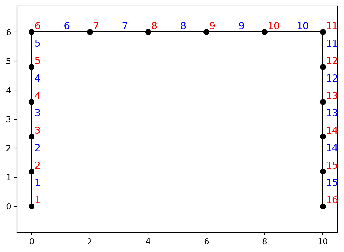
9.3.1 Nonlinear Response
A nonlinear analysis without sensitivity calculations is here conducted to see the load-displacement curve, for the displacement in the upper left corner of the frame:
dt = 0.05
nsteps = 20
t, lamda, u, void, void = nonlinearStaticAnalysis(structuralModel, nsteps, dt, trackNode, trackDOF)
plt.figure()
plt.plot(u, lamda, 'ko-')
plt.grid(True)
plt.xlabel("Displacement, $u$ [m]")
plt.ylabel("Load factor, $\\lambda$")
plt.show()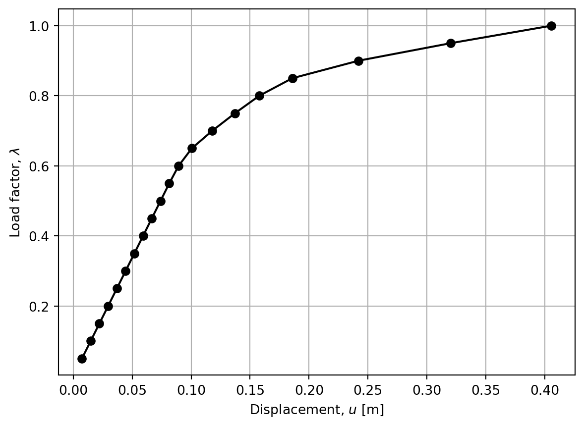
9.3.2 Response Statistics
Second-moment statistics for the input variables is provided in Listing 9.11. In total, there are 23 random variables. 21 are the different \(E\), \(f_y\), \(\alpha\), \(h_w\), \(b_f\), \(t_f\), and \(t_w\) in the beam and each of the two columns. In addition come the distributed load, \(q\), on the left-hand side column and the point load, \(F\), in the upper left corner of the frame. In Listing 9.11, response sensitivities are also requested for the 23 random variables. The analysis is re-run, now with sensitivity analysis. Notice that the model must be recreated to reset the value of the history variables in the material objects:
input = createNonlinearFrameInput(*means, nel)
structuralModel = model(input)
t, lamda, u, dudx, void = nonlinearStaticAnalysis(structuralModel, nsteps, dt, trackNode, trackDOF, DDMs, 1)
Now having response sensitivities, second-moment response statistics can be computed. In this case, second-order sensitivities are unavailable; hence, only the first-order mean is plotted, which is the displacement itself, shown as a black line:
covarianceMatrix = getCovMatrix(means, stdvs, correlation)
stdvFO = []
for n in range(len(t)):
    stdvFO.append(np.sqrt(dudx[:,n].dot(covarianceMatrix.dot(dudx[:,n]))))
stdvFO = np.array(stdvFO)
plt.figure()
plt.fill_betweenx(lamda, u-stdvFO, u+stdvFO, color='0.8')
plt.plot(u, lamda, 'k-', label='u')
plt.plot(u+stdvFO, lamda, 'b-', label='$u \\pm \\sigma_u$')
plt.plot(u-stdvFO, lamda, 'b-')
plt.grid(True)
plt.xlabel("Displacement")
plt.ylabel("Load factor")
plt.legend(loc='lower right')
plt.show()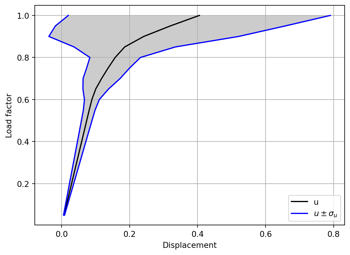
The plot above highlights a point made in the previous chapter; in the nonlinear response regime the standard deviation of the response can be very large.
9.3.3 Importance Ranking
The response sensitivities are here plotted:
plt.figure(); i=0
plt.plot(t, u, 'k-', label='u')
plt.plot(t, dudx[0,:]*stdvs[i], 'b-'); i+=1
plt.plot(t, dudx[1,:]*stdvs[i], 'b:'); i+=1
plt.plot(t, dudx[2,:]*stdvs[i], 'b--'); i+=1

plt.plot(t, dudx[3,:]*stdvs[i], 'r-'); i+=1
plt.plot(t, dudx[4,:]*stdvs[i], 'r:'); i+=1
plt.plot(t, dudx[5,:]*stdvs[i], 'r--'); i+=1

plt.plot(t, dudx[6,:]*stdvs[i], 'g-'); i+=1
plt.plot(t, dudx[7,:]*stdvs[i], 'g:'); i+=1
plt.plot(t, dudx[8,:]*stdvs[i], 'g--'); i+=1

plt.plot(t, dudx[9,:]*stdvs[i], 'c-'); i+=1
plt.plot(t, dudx[10,:]*stdvs[i], 'c:'); i+=1
plt.plot(t, dudx[11,:]*stdvs[i], 'c--'); i+=1

plt.plot(t, dudx[12,:]*stdvs[i], 'm-'); i+=1
plt.plot(t, dudx[13,:]*stdvs[i], 'm:'); i+=1
plt.plot(t, dudx[14,:]*stdvs[i], 'm--'); i+=1

plt.plot(t, dudx[15,:]*stdvs[i], 'y-'); i+=1
plt.plot(t, dudx[16,:]*stdvs[i], 'y:'); i+=1
plt.plot(t, dudx[17,:]*stdvs[i], 'y--'); i+=1

plt.plot(t, dudx[18,:]*stdvs[i], 'g-.'); i+=1
plt.plot(t, dudx[19,:]*stdvs[i], 'g-.'); i+=1
plt.plot(t, dudx[20,:]*stdvs[i], 'g-.'); i+=1

plt.plot(t, dudx[21,:]*stdvs[i], 'k:', label='$\\frac{\\partial u}{\\partial q}$'); i+=1
plt.plot(t, dudx[22,:]*stdvs[i], 'k--', label='$\\frac{\\partial u}{\\partial F}$')

plt.grid(True)
plt.xlabel("Pseudo time")
plt.ylabel("Importance, $\\frac{\\partial u}{\\partial x_i}\\cdot \\sigma_i$")
plt.legend(loc='upper left')
plt.show()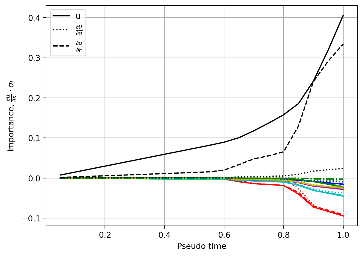
It is observed in the plot above that the point load, \(F\), is by far the most influential variable. A standard deviation increase in the value of that variable is predicted to double the final displacement. Naturally, \(\frac{\partial u}{\partial F}\) and \(\frac{\partial u}{\partial q}\), shown with black dashed and dotted lines, respectively, are positive. That means an increase in their value will increase the response. Conversely, the derivatives with respect to material and cross-section geometry variables are negative. Here is the same plot, now without \(u\), \(\frac{\partial u}{\partial F}\), and \(\frac{\partial u}{\partial q}\):
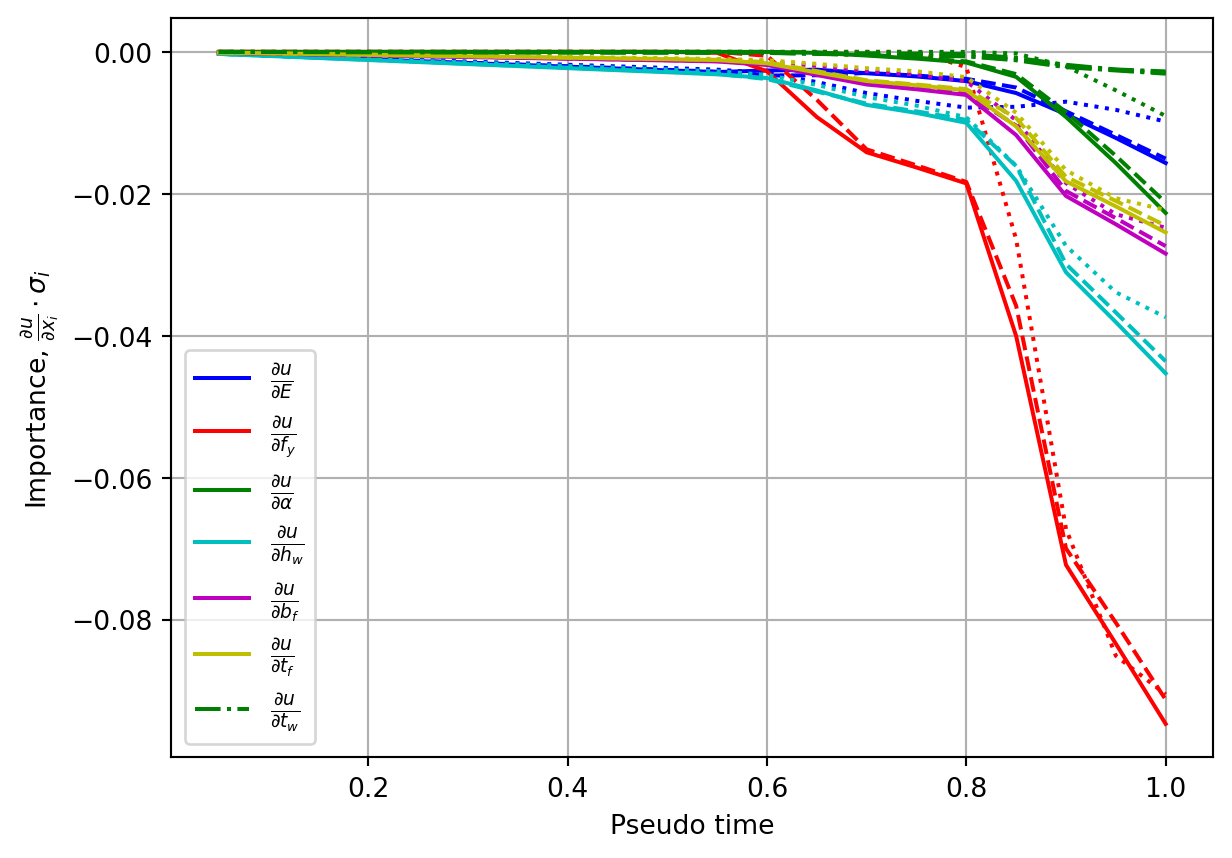
It is seen that, among the material and cross-section geometry variables, \(f_y\) is most important, followed by \(h_w\). Notice that the yield stress in the two columns, shown with solid and dashed lines, are more important than that in the beam (dotted line), early after yielding, indicating that the columns yield before the beam.
9.3.4 Reliability Analysis
A reliability analysis for the distributed plasticity nonlinear portal frame with 23 random variables is now carried out. To save computational time, 5 increments, each with \(\Delta t=0.2\), are employed to reach the \(\lambda=1\) load level. That is reflected in the following limit-state function, which makes use of information defined earlier in this chapter:
def nonlinearFrameLSF(x, threshold, needGradient=True):
    void, void, void, void, trackNode, trackDOF, DDMs = nonlinearFrameVariableSpecs(nel)
    nsteps = 5
    dt = 0.2
    input = createNonlinearFrameInput(*x, nel)
    structuralModel = model(input)
    void, void, u, dudx, void = nonlinearStaticAnalysis(structuralModel, nsteps, dt, trackNode, trackDOF, DDMs, 1)
    return (threshold-u[-1]), -dudx[:, -1]
The displacement threshold for which the exceedance probability is sought, in terms of \(\beta\), is the mean plus three standard deviations, using the first-order approximations calculated earlier:
threshold = u[-1] + 3 * stdvFO[-1]
beta, xStar, yStar, kappa = iHLRFalgorithm(nonlinearFrameLSF, threshold, means, stdvs, correlation, distributions, basicTransformation, False, True)
print(f"At threshold {threshold:.2f} the reliability index is {beta:.2f}")
HLRF step 1: Check1=1.00e+00,Check2=0.00e+00, y-norm=1.000
HLRF step 2: Check1=4.78e-01,Check2=3.05e-01, y-norm=3.000
HLRF step 3: Check1=1.71e-02,Check2=1.03e-01, y-norm=2.110
HLRF step 4: Check1=7.33e-04,Check2=8.35e-03, y-norm=2.127
iHLRF algorithm converged with beta=2.127
At threshold 1.56 the reliability index is 2.13The golden section line search algorithm for an optimal step size at each iteration of the HLRF algorithm was not activated here, still giving convergence in only a few iterations. Again, notice that the threshold “mean plus \(3\) standard deviations” is more likely to be exceeded than \(\beta=3\).