(More notes from Professor Terje Haukaas at terje.civil.ubc.ca.)

1  Introduction

The title of this book suggests that a structure can be sensitive. To boot, if you look at a constructed building or bridge, the title suggests that we can calculate how reliable it is. Both suggestions deserve a clarification, issued here at the outset.

First, this book adopts the definition that a sensitivity is a derivative. By sensitivity of a structure, we mean the derivative of one or more structural responses with respect to variables that define loading, material properties, and geometry. This book provides exact and efficiently computed first- and second-order sensitivities for all computational structural analysis types. Sensitivities can be examined for insight into structural behaviour, and they are invaluable in reliability analysis. In fact, this book conducts structural reliability analysis using exact first- and second-order response sensitivities for generic frame and truss structures.

Second, it is important to note that we will be dealing with structural models, not the real-world building or bridge. Therefore, when we talk about the reliability of a structure, then we mean the probability of events occurring within the confines of the idealized structural model. Moreover, those probabilities are founded on random variables that model uncertainties in the input variables. In contrast, uncertainties such as human error, which can also cause collapse of real-world structures, are not considered in this book.

1.1 Structural Models

The idealization of real-world structures is an art as well as a science. Different models may be appropriate, for the same structure, depending on the purpose of the model. A golden rule is to always be on the safe side; create a structural model that, if inaccurate, overestimates the structural response of interest. As a starting point, we limit the considerations to the common case of structures that lend themselves to a 2D idealized model. Next, the idealization process employs a “language” from which some terms are listed here:

1. Member types
   1. Truss members, carrying only axial force
   2. Beam/frame members, carrying bending moment, shear force, and axial force
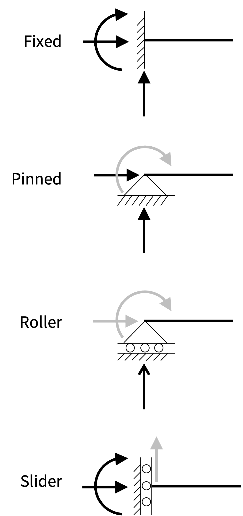
2. Support types (see Figure 1.1)
   1. Fixed
   2. Pinned
   3. Roller
   4. Slider
3. Degree of static indeterminacy (see Section 1.2)
   1. Minimize the number of member/reaction forces you rely on being actualized to carry the load considered

In regard to member and support types, the first rule is to be clear on which choices are made. That is, be conscious of the specific member and support types you select and make them clear in the drawing of the structural model. For example, a strong and stiff steel beam, which is clearly able to carry bending moment and shear force, may be considered as a truss member in your model. That is the case if its primary purpose, for the load considered, is to carry axial force.

The same goes for the choice of support type. Consider Figure 1.1, where the support types mentioned in the list above are visualized. The black arrows indicate the forces that are transferred into the foundation. Conversely, the white arrows are degrees of freedom (DOFs). The DOF concept is important in this book. For now, suffice to say that a DOF represents a displacement or rotation. In the same way that we may neglect the ability of a steel beam to carry moment and shear, we may neglect the ability of a support to carry a specific reaction force. We do that to be on the safe side, or to avoid counting on forces that are negligible or hard to actualize.

Figure 1.1: Support types in 2D structural models with reaction forces in black and degrees of freedom in white.

An example is a horizontal beam supported at both ends, analyzed in Chapter 15 and shown in Figure 15.1. When creating a model for that beam carrying distributed vertical load, it may be tempting to casually introduce a pinned support at each end. The next section will show that this is a statically indeterminate structure, which is awkward in this case. Because that model constrains the horizontal displacement at both ends, it says that the beam will start carrying the vertical load via axial tension, if the displacement becomes substantial. That is called the membrane effect in structural analysis.

It is possible to include that effect, but that is rarely meaningful for horizontal beams. Developing significant axial force in a beam to carry lateral load is difficult to achieve, regardless of how much concrete, reinforcing bars, or welds you ask the contractor to use. The correct structural model in this case is what we call a simply supported beam. That means a pinned support at one end and a roller at the other; it does not matter which is which. As will be seen in the next section, the simply supported beam adheres to Rule 3a in the list above by being statically determinate. In short, do not create a structural model that assumes that loads are carried by member or support forces that are either insignificant or hard to achieve.

1.2 Static Indeterminacy

Creating idealized structural models of real-world structures requires the consideration of degree of static indeterminacy (DSI). This concept is important also for a broader understanding of structural behaviour; hence, it deserves special attention. In basic structural analysis we learn that determinate structures, i.e., DSI=0 means that equilibrium considerations alone are sufficient for determining the internal force of the structure. Furthermore, DSI<0 means the structure is unstable and DSI>0 means that methods for indeterminate structures are needed, such as the flexibility and stiffness methods. More about structural analysis methods in the next section.

Textbooks on structural analysis employ different but equivalent ways of counting the DSI. It is possible to utilize the DOF concept mentioned above. It is also possible to “cut” the structure in different ways to reach a determinate structure, letting the number of cuts reflect the DSI. For any given structural model, there is only one correct answer to what the DSI is. Informally, it is

DSI= Number of unknown forces - Number of equations and releases

More formally, the following formula is employed in this book:

\[ DSI = (f \cdot m + s ) - (e \cdot j + h) \tag{1.1}\]

where \(f=\) number of unknown forces in each member, addressed shortly with the help of Table 1.1, \(m=\) number of members of the type \(f\) is representative of, \(s=\) number of support reactions, \(e=\) number of equations per joint, again with reference to Table 1.1, \(j=\) number of joints of the type that \(e\) refers to, and \(h=\) number of hinges, or more precisely the number of releases of member forces.

Table 1.1 correctly suggests that the axial force is the single internal force, \(f\) in a 2D truss member. The 2D frame element has three: axial force, bending moment, and shear force. Table 1.1 also counts the \(e=2\) equilibrium equations we count at a joint where only truss members enter, i.e., horizontal and vertical equilibrium. A joint in a 2D structure where one or more beam/frame members enter has \(e=3\) because then we include rotational equilibrium.

Table 1.1: \(f\) and \(e\) for calculation of DSI.

Member/structure type	\(f\)	\(e\)
2D truss	1	2
2D frame	3	3
3D truss	1	3
3D frame	6	6

Step by step, through the chapters of this book, a Python library for reliability and sensitivity analysis of structures is assembled. The code addresses linear and nonlinear problems, both static and dynamic. Truss and frame structures with varying complexity are considered, and varous element, cross-section, and material options will be introduced.

The first look at the input format for that code is provided below in Listing 1.1. Without the details introduced in subsequent chapters, it specifies a simply supported beam, like the one described in the previous section. For readers unfamiliar with the concepts of nodes and elements, the next section will help. The input below gives \((x, y)\) coordinates for two nodes, one at each end of the element. The values seen in the NODES array give a 4m length of the beam. The CONSTRAINTS array says that the left-hand side node is pinned because the two first DOFs have 1=fixed and the third has 0=free. In this book, the DOF numbering is

1. Horizontal displacement
2. Vertical displacement
3. Rotation

That means the right-hand side node is a roller because only the vertical DOF is restrained. Listing 1.1 does not provide details on cross-section and material properties for the column. However, the elementType variable is necessary to tell if the element is a truss or frame member. In this book all truss members have numbers below 5, with elementType = 5 representing the linear elastic frame element introduced in Chapter 3. Together with that information, the ELEMENTS array given below simply says that a single element connects Node 1 and Node 2:

Listing 1.1: Structural model for vertical cantilever.

NODES = [[0.0, 0.0],
         [4.0, 0.0]]

CONSTRAINTS = [[1, 1, 0],
               [0, 1, 0]]
elementType = 5
ELEMENTS = [[elementType, 1, 2]]

The Python function defined below calculates the DSI for generic input given by NODES, CONSTRAINTS, and ELEMENTS. For brevity, checking the input is postponed until later chapters. Examining the code in Listing 1.2 reveals that the formula in Equation 1.1 is employed. The code iterates over the NODES, CONSTRAINTS, and ELEMENTS arrays to collect the terms of that formula:

Listing 1.2: Algorithm for calculating DSI.

def calculateDSI(NODES, CONSTRAINTS, ELEMENTS):

    # Formula: DSI = (f*m + s) - (e*j + h)

    # Loop over elements to determine f*m
    fm = 0
    for i in range(len(ELEMENTS)):
        if ELEMENTS[i][0] < 5: # Truss elements
            fm += 1
        else:                  # Frame elements
            fm += 3

    # Loop over nodes to determine e*j
    ej = 0
    for i in range(len(NODES)):
        e = 2
        for j in range(len(ELEMENTS)):
            # Check if Element j connects to Node i:
            if ELEMENTS[j][-1]==i+1 or ELEMENTS[j][-2]==i+1:
                if ELEMENTS[j][0] > 4: # If frame element
                    e = 3
        ej += e

    # Number of support reactions, s
    s = sum(sum(row) for row in CONSTRAINTS)

    # No hinge option for now
    h = 0

    # Calculate DSI
    dsi = (fm + s) - (ej + h)

    # Print the result
    print("The calculation gives DSI = %.i." % dsi)

    return dsi

The result of running the calculateDSI() function defined in Listing 1.2 for the simply supported beam defined in Listing 1.1 is shown here:

dsi = calculateDSI(NODES, CONSTRAINTS, ELEMENTS)

The calculation gives DSI = 0.

Naturally, the result shows that the simply supported beam is statically determinate. Perhaps you want to check that the pinned-pinned input CONSTRAINTS = [[1, 1, 0], [1, 1, 0]] discussed in the previous section gives an indeterminate structure.

1.3 Portal Frame Example

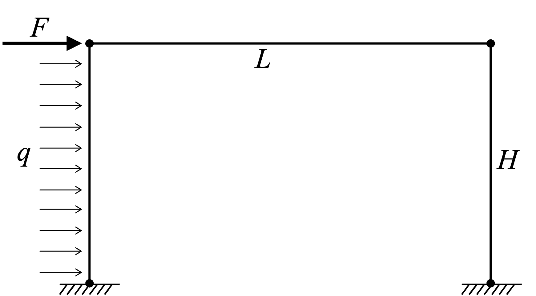
In several chapters of this book, a portal frame with fixed support at the base of the columns will serve as demonstration example. Figure 1.2 shows this structure, together with the definition of symbols for loads and dimensions.

Figure 1.2: Portal frame example.

Below, the first simple model of that frame is created, for now without loads and other details:

Listing 1.3: Structural model for portal frame.

NODES = [[0.0,  0.0],
         [0.0,  6.0],
         [10.0, 6.0],
         [10.0, 0.0]]

CONSTRAINTS = [[1, 1, 1],
               [0, 0, 0],
               [0, 0, 0],
               [1, 1, 1]]
elementType = 5
ELEMENTS = [[elementType, 1, 2],
            [elementType, 2, 3],
            [elementType, 3, 4]]

dsi = calculateDSI(NODES, CONSTRAINTS, ELEMENTS)

The calculation gives DSI = 3.

The calculation in the last line of that code shows that the fixed-fixed portal frame in Figure 1.2 is indeterminate to the third degree. That result is verified by the approach adopted in some textbooks: Suppose we completely cut the horizontal beam that connects the columns. That means enforcing zero moment, shear, and axial force at that location. Having “cut” those three internal forces, we are left with two separate statically determinate cantilevers, confirming that DSI=3 is correct.

1.4 Structural Analysis Methods

Taking part in a fascinating human activity, structural engineers design much of our built environment. Being a structural engineer means utilizing codes, standards, mathematical equations, computer analysis, practical experience, and judgment. It also means considering the utility of the structure and the impacts of its construction. To explain the role of structural analysis in this, we say that

Structural Engineering = Design + Analysis

This means structural engineering is a back-and-forth between design and analysis. Specifically, the engineer establishes a candidate design, followed by structural analysis. The analysis aims to determine deformations and internal forces in the structure. The internal forces include bending moments, shear forces, axial forces, reaction forces, and possibly torque in members. The relevant structural responses are then examined to judge if the design is adequate, or if the engineer needs to modify the design. Delving deeper into the structural analysis portion, we say that

Structural Analysis = Models + Methods

The structural models are addressed earlier in this chapter; attention is now turned to the structural analysis methods. For the truss and frame structures considered in this book, this is a list of viable methods:

• Deformations
  • Unit virtual force method
  • Moment area method
  • Conjugate beam method
  • Solving differential equation
• Internal forces
  • Equilibrium alone
  • Flexibility method
  • Stiffness method
  • Slope-deflection method
  • Moment distribution method
  • Matrix structural analysis
  • Finite element method
  • Approximate analysis

Even after limited exposure to engineering education, we are familiar with several of these methods. As mentioned earlier, equilibrium alone is sufficient for finding internal forces when DSI=0. Conversely, for indeterminate structures, we often learn the flexibility method first. However, relevant for this book is that the flexibility method is inconvenient for implementation on the computer.

Instead, it is the stiffness method that forms the basis for computer implementation of structural analysis. It is a displacement-based method, which means that displacements and rotations are the primary unknowns. Indeed, such methods provide deformations as well as internal forces. This contrasts with the flexibility method, where forces are the primary unknowns. While those unknown forces must be selected subjectively, the unknown displacements and rotations in displacement-based methods, i.e., DOFs can be systematically determined by a computer.

In the list provided above, the stiffness method, slope-deflection method, moment distribution method, matrix structural analysis, and the finite element method are all displacement-based methods with common characteristics. That said, moment distribution and the slope-deflection method are meant for hand calculations. In the context of computational analysis, the stiffness method, matrix structural analysis, and the finite element method are applicable and closely related.

1.5 Degrees of Freedom

The unknown displacements and rotations in a structural analysis are earlier labelled DOFs. In the upper left corner, Figure 1.3 shows the three DOFs for a cantilevered column. Positive rotation is consistently clockwise in figures and equations throughout this book. However, for legacy reasons, you will in this version of the book find positive counterclockwise rotation in certain locations in the Python code.

The DOFs for the fixed-fixed portal frame defined earlier in Listing 2.1 are show in the top centre of Figure 1.3. Again, we notice three DOFs at every node, in this case meaning both corners of the frame. If the bottom nodes were not completely fixed, but allowed to rotate, then the top right configuration in Figure 1.3 is correct. Specifically, rotational DOFs at the base reflect the possibility of rotation there.

Figure 1.3: Degrees of freedom in 2D truss, frame, and mixed structural models.

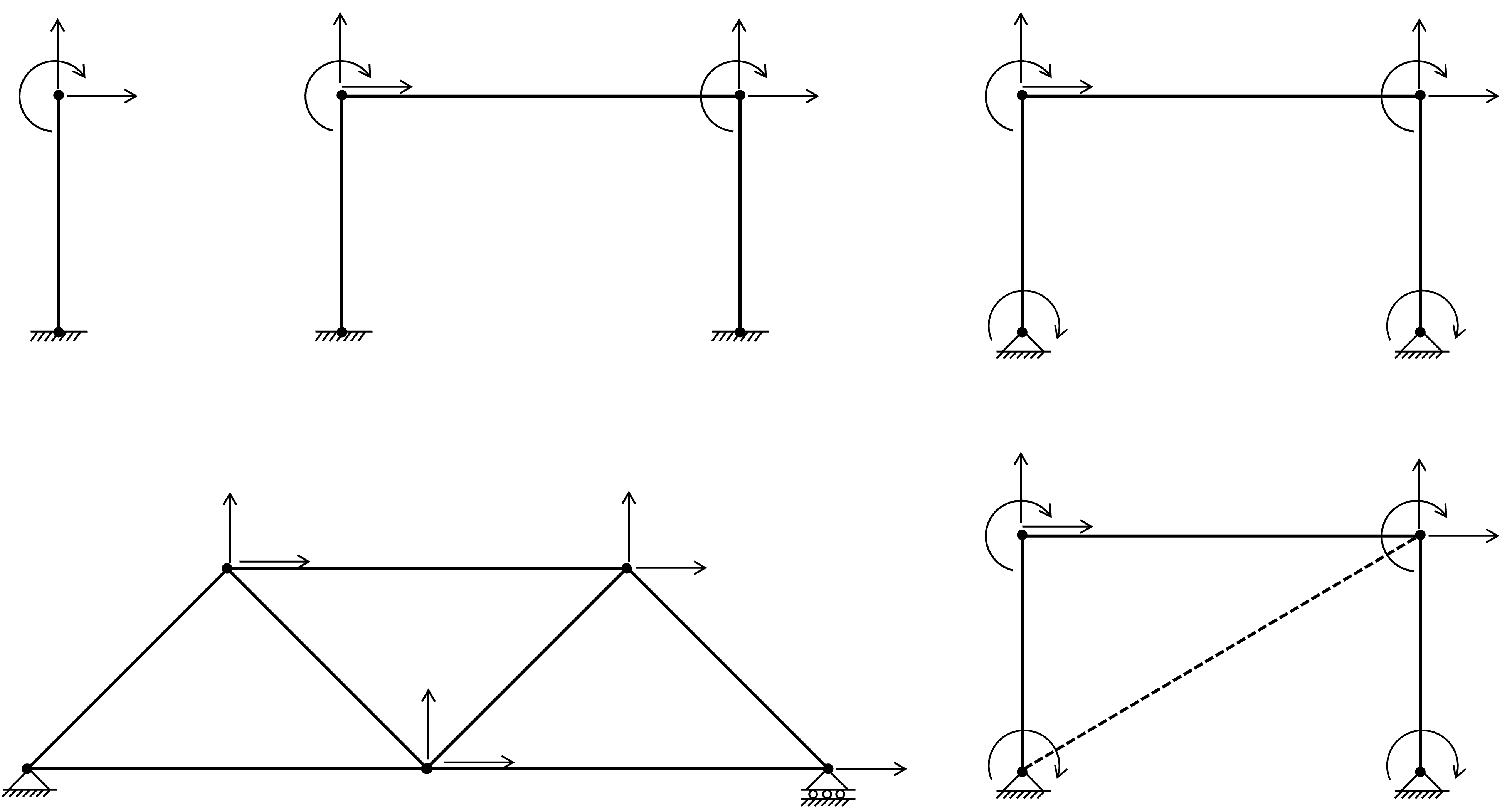
The bottom left of Figure 1.3 shows a truss structure, to highlight that no rotational DOFs are present in a pure truss. Naturally, this means that the pinned support on the left-hand side of that truss does not have any DOFs, while the roller on the right-hand side has one DOF. The bottom right of Figure 1.3 shows a frame that has a dashed truss member serving as bracing. Although a truss member is here present, the default is three DOFs per node for such mixed structures. To follow up on that point, if a mixed structure has one or more nodes with only truss members connected to it, then the rotational DOF of such nodes must be fixed because that DOF has zero stiffness, meaning it is unstable.

Same as the counting of DSI, the selection of DOFs has only one correct answer in the computational approach. This is why displacement-based methods are well suited for computer analysis. We simply specify nodal coordinates, boundary conditions, and element connectivity, and the computer figures out the DOFs. Matching the abbreviation DSI, we may refer to the number of DOFs by the abbreviation DKI, i.e., degree of kinematic indeterminacy. Both DSI and DKI are independent of the loading that is applied to the structure.

1.6 Response Equations

Those familiar with the flexibility method of structural analysis will recall that kinematic compatibility forms the governing equations for the unknown forces. Conversely, in displacement-based methods we establish equilibrium equations to solve for DOFs. For a single elastic spring, fixed at one end with a force, \(F\), at the other end, equilibrium reads

\[ Ku=F \tag{1.2}\]

where \(K=\) stiffness coefficient of the spring and \(u=\) displacement at the free end of the spring. That simple example is the basis for the following notation for the governing response equations for a structural model with two DOFs:

\[ \begin{aligned} K_{11}\cdot u_1 + K_{12}\cdot u_2 &= F_1 \\ K_{21}\cdot u_1 + K_{22}\cdot u_2 &= F_2 \end{aligned} \tag{1.3}\]

In the multi-DOF case, \(K_{ij}=\) force along DOF \(i\) due to a unit displacement along DOF \(j\). In matrix form, those equilibrium equations are written

\[ \mathbf{K} \mathbf{u} = \mathbf{F} \tag{1.4}\]

where \(\mathbf{K}=\) square symmetric positive definite matrix with dimension equal to the number of DOFs, \(\mathbf{u}=\) displacement vector, i.e., the vector of displacements and rotations along the DOFs, and \(\mathbf{F}=\) load vector that introduces the external loads on the structure. In this book, \(\mathbf{u}\) is the structural response considered at first. However, it is straightforward to determine the internal forces in the members of a structure from \(\mathbf{u}\). Details on that are provided in subsequent chapters. For those seeking further distinctions between the displacement-based methods of computational structural analysis, this is offered:

• Stiffness method = methodological foundation, employed also in hand calculations, but then often with axial deformations neglected, unless the structure is a truss
• Matrix structural analysis = techniques for establishing \(\mathbf{K}\) and \(\mathbf{F}\) by assembling contributions from individual elements
• Finite element method = an approach for establishing \(\mathbf{K}\) and \(\mathbf{F}\) for individual elements, including plates and shells, via integration, sometimes with approximate results

In subsequent chapters, five structural analysis types are explained, extended, and applied:

• Linear static analysis
• Nonlinear static analysis
• Linear multi-DOF dynamic analysis
• Nonlinear single-DOF dynamic analysis
• Nonlinear multi-DOF dynamic analysis

The first option has Equation 1.4 as its governing response equations; the other analysis types are extensions of that. The most general version, applicable to nonlinear multi-DOF dynamic analysis, is \[ \mathbf{M} \ddot{\mathbf{u}} + \mathbf{C}\dot{\mathbf{u}} + \tilde{\mathbf{F}}(\mathbf{u}) = \mathbf{F}(t) \tag{1.5}\]

where \(\mathbf{M}=\) mass matrix, \(\ddot{\mathbf{u}}=\) acceleration vector, \(\mathbf{C}=\) damping matrix, \(\dot{\mathbf{u}}=\) velocity vector, and \(\tilde{\mathbf{F}}(\mathbf{u})=\) are the forces that the structure is resisting displacements with. Shown in derivations later in this book, the first term in Equation 1.5 represents inertia forces, the second term represents viscous damping forces, and the remaining two terms represent Equation 1.4. That means \(\tilde{\mathbf{F}}(\mathbf{u})\) replaces \(\mathbf{Ku}\) in nonlinear analysis. The time-varying load in the right-hand side of Equation 1.5 is in this book defined by ground motion, as described in Section 10.10.

1.7 Sensitivity Equations

A first-order response sensitivity of interest in this book is \(\frac{\partial \mathbf{u}}{\partial \mathbf{x}}\). Usually containing material, geometry, and load variables, \(\mathbf{x}\) is a vector of input variables to the structural model. Because \(\mathbf{x}\) and \(\mathbf{u}\) are both vectors, the response sensitivity \(\frac{\partial \mathbf{u}}{\partial \mathbf{x}}\) is a matrix. However, often we seek just one component or a slice of that matrix, such as the derivative of a single structural response, \(u\), selected from \(\mathbf{u}\), i.e., \(\frac{\partial u}{\partial \mathbf{x}}\).

At this point in the introduction, we are not modelling the uncertainty in the input variables, \(\mathbf{x}\). However, we are interested in the change in the structural response caused by a change in the value of one or more of the input variables.

The derivation/implementation of first-order response sensitivities differs for the analysis types listed in the previous section. However, common to all analysis types is the direct differentiation method (DDM) employed in this book. That approach entails analytical differentiation of the governing response equations, followed by their implementation inside the structural analysis algorithm. The DDM contrasts with finite difference methods, which require at least one new structural analysis for every variable in \(\mathbf{x}\) to obtain approximate sensitivities. The DDM calculates exact response sensitivities, efficiently alongside the response, in one analysis.

Diffent chapters in this book explain the implementation details for each analysis type. The basic concepts of the DDM are here outlined by considering the linear elastic problem in Equation 1.4. In this context it is pedagogical to consider the case of a single input variable, \(x\). To that end, we rewrite the governing response equations by acknowledging dependencies on \(x\):

\[ \mathbf{K}(x) \mathbf{u}(x) = \mathbf{F}(x) \tag{1.6}\]

It is reiterated that \(x\) is a load or a material or cross-section property. It is not certain that \(x\) affects all quantities in Equation 1.6. However, for generality, we keep the notation \(\mathbf{K}(x)\) and \(\mathbf{F}(x)\), although one of them may ultimately be independent of \(x\), and thus its derivative zero. Differentiating Equation 1.6 with respect to \(x\) yields, via the product rule of differentiation, \[ \frac{\partial \mathbf{K}}{\partial x} \mathbf{u} + \mathbf{K} \frac{\partial \mathbf{u}}{\partial x} = \frac{\partial \mathbf{F}}{\partial x} \tag{1.7}\]

Rearranging yields a linear system of equations with coefficient matrix identical to Equation 1.4: \[ \mathbf{K} \frac{\partial \mathbf{u}}{\partial x} = \frac{\partial \mathbf{F}}{\partial x} - \frac{\partial \mathbf{K}}{\partial x} \mathbf{u} \tag{1.8}\]

Only the right-hand side differs between Equation 1.4 and Equation 1.8. That means the equation solvers utilized to solve Equation 1.4 are employed to solve Equation 1.8. In fact, decomposition and back-substitution techniques used by the solver for Equation 1.4 benefit the repeated solving of Equation 1.8 to determine the response sensitivity \(\frac{\partial \mathbf{u}}{\partial x}\). This book confirms a fact pointed out by Zhang and Der Kiureghian (1993): Regardless of structural analysis type, even for nonlinear dynamic problems, response sensitivities are solved from a linear system of equations, without iterations, once the structural response is determined.

The same holds true for the calculation of second-order response sensitivities. To differentiate Equation 1.7, it is helpful to introduce index notation to separate the \(x\)-variable in the first differentiation from the \(x\)-variable in the second. Those two input variables may be the same, but they may also be different, yielding cross-derivatives. The notation \(x_i\) and \(x_j\) is employed, with \(i\) and \(j\) counting over the number of input variables in \(\mathbf{x}\). Differentiation of Equation 1.7 gives

\[ \phantom{{}+{}}\frac{\partial^2 \mathbf{K}}{\partial x_i \partial x_j} \mathbf{u} + \frac{\partial \mathbf{K}}{\partial x_i} \frac{\partial \mathbf{u}}{\partial x_j} + \frac{\partial \mathbf{K}}{\partial x_j} \frac{\partial \mathbf{u}}{\partial x_i} + \mathbf{K} \frac{\partial^2 \mathbf{u}}{\partial x_i \partial x_j} = \frac{\partial^2 \mathbf{F}}{\partial x_i \partial x_j} \tag{1.9}\]

Solving for the sought second-order response sensitivity again yields a linear system of equations:

\[ \mathbf{K} \frac{\partial^2 \mathbf{u}}{\partial x_i \partial x_j} = \frac{\partial^2 \mathbf{F}}{\partial x_i \partial x_j} - \frac{\partial^2 \mathbf{K}}{\partial x_i \partial x_j} \mathbf{u} - \frac{\partial \mathbf{K}}{\partial x_i} \frac{\partial \mathbf{u}}{\partial x_j} - \frac{\partial \mathbf{K}}{\partial x_j} \frac{\partial \mathbf{u}}{\partial x_i} \tag{1.10}\]

It is reiterated that the response must be obtained from Equation 1.4 before Equation 1.8 is solved for first-order sensitivities. Similarly, first-order sensitivities must be obtained from Equation 1.8 before Equation 1.10 is solved for second-order sensitivities. This procedure is observed in the code presented later in this book.

1.8 Adjoint Method

In structural analysis we are often interested in just one, or a few, displacement responses. For example, in the next few chapters of this book, the displacement, \(u\), at the upper left corner of the frame in Figure 1.2 serves as the response of interest. In such circumstances the adjoint method may bring computational savings to the sensitivity calculations. To understand this, consider the calculation of \(\frac{\partial u}{\partial x}\) in linear static analysis. The sought derivative is first expanded using the chain rule of differentiation: \[ \frac{\partial u}{\partial x} = \frac{\partial u}{\partial \mathbf{u}}\frac{\partial \mathbf{u}}{\partial x} \tag{1.11}\]

The first factor in the product on the right-hand side is a vector of zeros, except a unit value in the position of \(\mathbf{u}\) that \(u\) is taken from. That vector is here labelled a selection vector: \(\mathbf{s} \equiv \frac{\partial u}{\partial \mathbf{u}}\). Next, in an operation that is never executed, the second factor on the right-hand side is expressed as the solution to Equation 1.8 like this:

\[ \frac{\partial \mathbf{u}}{\partial x} = \mathbf{K}^{-1}\left(\frac{\partial \mathbf{F}}{\partial x} - \frac{\partial \mathbf{K}}{\partial x} \mathbf{u}\right) \tag{1.12}\]

Substitution of \(\mathbf{s}\) and Equation 1.12 into Equation 1.11 yields: \[ \frac{\partial u}{\partial x} = \mathbf{s} \mathbf{K}^{-1}\left(\frac{\partial \mathbf{F}}{\partial x} - \frac{\partial \mathbf{K}}{\partial x} \mathbf{u}\right) \tag{1.13}\]

Outside the parenthesis in the right-hand side of Equation 1.13 is the quantity \(\mathbf{s} \mathbf{K}^{-1}\), which is worth giving a name: \[ \pmb{\lambda} \equiv \mathbf{s} \mathbf{K}^{-1} \tag{1.14}\]

We never establish the inverse of the stiffness matrix; however, the vector \(\pmb{\lambda}\) is efficiently solved from the linear system of equations expressed in this rearranged version of Equation 1.14:

\[ \mathbf{K} \pmb{\lambda} \equiv \mathbf{s} \tag{1.15}\]

Once \(\pmb{\lambda}\) is determined by solving Equation 1.15 once and for all, \(\frac{\partial u}{\partial x}\) is determined for any number of \(x\)-variables simply by a dot product:

\[ \frac{\partial u}{\partial x} = \pmb{\lambda} \left(\frac{\partial \mathbf{F}}{\partial x} - \frac{\partial \mathbf{K}}{\partial x} \mathbf{u}\right) \tag{1.16}\]

In the same way that the dot product in Equation 1.16 solves the linear system of equations in Equation 1.8, the dot product \[ \frac{\partial^2 u}{\partial x_i \partial x_j} = \pmb{\lambda} \left(\frac{\partial^2 \mathbf{F}}{\partial x_i \partial x_j} - \frac{\partial^2 \mathbf{K}}{\partial x_i \partial x_j} \mathbf{u} - \frac{\partial \mathbf{K}}{\partial x_i} \frac{\partial \mathbf{u}}{\partial x_j} - \frac{\partial \mathbf{K}}{\partial x_j} \frac{\partial \mathbf{u}}{\partial x_i} \right) \tag{1.17}\]

solves Equation 1.10 for second-order response sensitivites. However, the adjoint method has limitations:

• It cannot be applied consecutively to calculate the response, then first-order sensitivities, and ultimately second-order sensitivities. That is because the parenthesis in Equation 1.16 requires the full displacement response vector, \(\mathbf{u}\), not only \(u\), and the parenthesis in Equation 1.17 requires the full first-order sensitivity vector, \(\frac{\partial \mathbf{u}}{\partial x}\), not only \(\frac{\partial u}{\partial x}\). That is why, if response sensitivities are sought, the adjoint method is applied only in the last calculations. Specifically, if second-order sensitivities are sought, then the adjoint method is applied only to Equation 1.17. Conversely, if only first-order sensitivities are sought, then the adjoint method is applied to Equation 1.16.

• If the sensitivity of element responses, such as bending moments and shear forces, are sought then the elements need to receive \(\frac{\partial \mathbf{u}}{\partial x}\) for all its DOFs, making the adjoint method inapplicable.

• In nonlinear static or dynamic analysis, with hysteretic material models, the derivative of all history variables must be stored for subsequent load steps. In order to accomplish this, the elements need to receive \(\frac{\partial \mathbf{u}}{\partial x}\) for all its DOFs, which again makes the adjoint method inapplicable.

1.9 Structural Reliability

The word reliability is not casually employed in this book. It comes with a specific definition that yields a scalar number as result. While the reliability of a structure is not given a dedicated symbol, its complement is:

\[ \begin{aligned} \mathrm{Reliability} &= 1- \mathrm{P}[\mathrm{Failure}] \\ &\equiv 1 - p_f \end{aligned} \tag{1.18}\]

where \(\mathrm{P}[\cdot]\) is the probability operator and “Failure” is an event. Essentially, the event that a structure is reliable is the complement of the event that it fails. This is why subsequent chapters present methods for calculating \(p_f\), still under the headline reliability analysis. However, we have great flexibility in defining the failure event. For example, we may seek the probability that the displacement at a particular location in the structure exceeds a threshold. That means we can define “failure” as \(u(\mathbf{x})\) exceeding, say, 0.025mm although that event may come with insignificant adverse effects for the structure.

Broadly speaking, a structural reliability problem has two ingredients, addressed in the next two sections:

• One or more limit-state functions that employ one or more structural responses to define what is considered failure
• Random variables that model uncertainty in the input variables

1.10 Limit-state Functions

It is the concept of a limit-state function, denoted by \(g(\mathbf{x})\), that allows us to define the failure event that we seek the probability of in a reliability analysis. In the literature, the following convention for \(g(\mathbf{x})\) is generally accepted:

• \(g(\mathbf{x}) \leq 0\) means failure
• \(g(\mathbf{x}) > 0\) means safe
• \(g(\mathbf{x}) = 0\) is the boundary between the “failure domain” in the space of \(\mathbf{x}\) variables and the safe domain; this boundary is sometimes called the limit-state surface

In the text above, the example of seeking the probability that a certain displacement exceeds 0.025m is mentioned. The corresponding limit-state function is

\[ g(\mathbf{x}) = 0.025 - u(\mathbf{x}) \tag{1.19}\]

Notice that \(g\) is negative when \(u\) exceeds 0.025m, thus conforming to the convention given above. Of equal importance in this book is that \(g(\mathbf{x})\), such as the one in Equation 1.19, is practically always a nonlinear function of \(\mathbf{x}\). One may think that the function \(u(\mathbf{x})\) is linear for linear structural analysis. However, proportionality between applied load and resulting displacement does not mean that \(u\) is a linear function of \(\mathbf{x}\). This is apparent in the simplest of structural analysis problems. Even when calculating the displacement at the midspan of a simply supported beam we observe the beam length appearing to the power of 3 or 4, depending on the loading, with the bending stiffness in the denominator. Hence, they both affect the displacement in a nonlinear manner. This is why the two-variable linear limit-state function \(g(\mathbf{x}) = R - S\), common in textbooks on reliability analysis, is irrelevant in this book.

1.11 Random Variables

The cornerstone of uncertainty modelling in this book is to consider the input variables, \(\mathbf{x}\), as random variables. Specifically, we consider them to be continuous random variables. This book employs the symbol \(x\) and \(\mathbf{x}\) for both the random variables and their realizations. This is mentioned because some literature, such as the seminal textbook by Der Kiureghian (2022), reserves upper-case for the random variable and lower-case for its outcome. In that case, an upper-case subscript is attached to each probability distribution to name the random variable it is the distribution for. For the applications considered in this book, relying solely on lower-case is unambiguous.

One way of characterizing the uncertainty in a variable, \(x\), is to specify its probability distribution. Here considering the distribution for individual variables, i.e., marginal distributions, they come in three related forms:

• Probability density function (PDF):

\[ f(x)=\frac{dF(x)}{dx}=-\frac{dG(x)}{dx} \tag{1.20}\]

• Cumulative distribution function (CDF):

\[ F(x)=\int_{-\infty}^{x} f(x) \,dx = 1-G(x) \tag{1.21}\]

• Complementary cumulative distribution function (CCDF):

\[ G(x)=1-\int_{-\infty}^{x} f(x) \,dx = 1-F(x) \tag{1.22}\]

An additional representation is the inverse CDF, i.e., \(F^{-1}(p)\). That does not mean inverse in the sense \(1/F(x)\) but inverse in the same way we employ \(\mathrm{tan}^{-1}(x)\) in trigonometry. A number of standard distribution types exist for continuous random variables, including

• Normal
• Lognormal
• Uniform
• Exponential
• Gamma
• Rayleigh
• Beta
• Chi-squared
• Weibull
• Logistic

Each distribution type has one or more model parameters. The Normal distribution has the two parameters \(\mu\) and \(\sigma\), representing the mean and standard deviation, respectively. In fact, lack of data to support a specific distribution type, or benefits to analysis procedures and interpretation of results, sometimes lead us to use only \(\mu\) and \(\sigma\).

To that end, let us look closer at \(\mu\) and \(\sigma\). In this introduction, we review the concept of statistical moments for continuous probability distributions. Similar to the first moment of area and moment of inertia in cross-section analysis, statistical moments are integrals. The symbols employed in Table 1.2 show that the mean, \(\mu\), is the first statistical moment of a random variable.

It is also shown in Table 1.2 that the standard deviation, \(\sigma\), is the square root of the second central statistical moment, which is called the variance. In regard to the other two integrals in Table 1.2, the first central moment is always zero, just like the first moment of area of an entire cross-section is zero when the axes originate at its centroid. The centroid of cross-sections is conceptually equivalent to the mean of a random variable. The second statistical moment in Table 1.2 is called the mean square of the distribution but is not given a symbol.

Table 1.2: Statistical moments.

	Moments	Central moments
First-order	\(\mu=\int_{-\infty}^{\infty} x\cdot f(x) \,dx\)	\(\int_{-\infty}^{\infty} (x-\mu)\cdot f(x) \,dx\)
Second-order	\(\int_{-\infty}^{\infty} x^2 \cdot f(x) \,dx\)	\(\sigma^2=\int_{-\infty}^{\infty} (x-\mu)^2 \cdot f(x) \,dx\)

When we consider joint, i.e., multivariate probability distributions for a vector of variables, \(\mathbf{x}\), then the concept of correlation is relevant. The correlation coefficient for two random variables \(x_i\) and \(x_j\) is a number between \(-1\) and \(1\):

\[ \rho_{ij} = \frac{\mathrm{Cov}[x_i, x_j]}{\sigma_i \cdot \sigma_j} = \frac{\int_{-\infty}^{\infty} \int_{-\infty}^{\infty} (x_i-\mu_i) \cdot (x_j-\mu_j) \cdot f(x_i, x_j) \,dx_i \,dx_j}{\sigma_i \cdot \sigma_j} \tag{1.23}\]

where \(f(x_i, x_j)\) is the joint PDF. The numerator is the covariance, which is another second-order moment. This is why an analysis that employs only \(\mu\), \(\sigma\), and \(\rho\) for the random variables is referred to as second-moment analysis. As shown later in this book, the second-moment approach delivers powerful and transparent response statistics and reliability methods. It is common to express the standard deviation of a random variable via the coefficient of variation:

\[ \delta = \frac{\sigma}{\mu} \tag{1.24}\]

In this way, a 10% coefficient of variation, i.e., \(\delta=0.1\) means that the standard deviation is 10% of the mean. Also, in the development of second-moment methods, the information given in Table 1.2 and Equation 1.23 is collected in vector-matrix form. The mean vector is \[ \pmb{\mu} = \begin{Bmatrix} \mu_1 \\ \mu_2 \\ \mu_3 \\ \vdots \\ \mu_N \end{Bmatrix} \tag{1.25}\]

where \(N=\) number of random variables. The correlation matrix,

\[ \mathbf{R} = \begin{bmatrix} 1 & \rho_{12} & \rho_{13} & \cdots & \rho_{1N} \\ \rho_{21} & 1 & \rho_{23} & \cdots & \rho_{2N} \\ \rho_{31} & \rho_{32} & 1 & \cdots & \rho_{3N} \\ \vdots & \vdots & \vdots & & \vdots \\ \rho_{N1} & \rho_{N2} & \rho_{N3} & \cdots & 1 \end{bmatrix} \tag{1.26}\]

is symmetric, which is also a property of the covariance matrix:

\[ \begin{aligned} \pmb{\Sigma} &= \begin{bmatrix} \sigma_1^2 & \mathrm{Cov}[x_1, x_2] & \mathrm{Cov}[x_1, x_3] & \cdots & \mathrm{Cov}[x_1, x_N] \\ \mathrm{Cov}[x_2, x_1] & \sigma_2^2 & \mathrm{Cov}[x_2, x_3] & \cdots & \mathrm{Cov}[x_2, x_N] \\ \mathrm{Cov}[x_3, x_1] & \mathrm{Cov}[x_3, x_2] & \sigma_3^2 & \cdots & \mathrm{Cov}[x_3, x_N] \\ \vdots & \vdots & \vdots & & \vdots \\ \mathrm{Cov}[x_N, x_1] & \mathrm{Cov}[x_N, x_2] & \mathrm{Cov}[x_N, x_3] & \cdots & \sigma_N^2 \end{bmatrix} \\ \\ &= \begin{bmatrix} \sigma_1^2 & \rho_{12}\sigma_1\sigma_2 & \rho_{13}\sigma_1\sigma_3 & \cdots & \rho_{1N}\sigma_1\sigma_N \\ \rho_{21}\sigma_2\sigma_1 & \sigma_2^2 & \rho_{23}\sigma_2\sigma_3 & \cdots & \rho_{2N}\sigma_2\sigma_N \\ \rho_{31}\sigma_3\sigma_1 & \rho_{32}\sigma_3\sigma_2 & \sigma_3^2 & \cdots & \rho_{3N}\sigma_3\sigma_N \\ \vdots & \vdots & \vdots & & \vdots \\ \rho_{N1}\sigma_N\sigma_1 & \rho_{N2}\sigma_N\sigma_2 & \rho_{N3}\sigma_N\sigma_3 & \cdots & \sigma_N^2 \end{bmatrix} \end{aligned} \tag{1.27}\]

For certain derivations later in this book it is helpful to define the diagonal matrix that has the standard deviations on the diagonal:

\[ \mathbf{D} = \begin{bmatrix} \sigma_1 & 0 & 0 & \cdots & 0 \\ 0 & \sigma_2 & 0 & \cdots & 0 \\ 0 & 0 & \sigma_3 & \cdots & 0 \\ \vdots & \vdots & \vdots & & \vdots \\ 0 & 0 & 0 & \cdots & \sigma_N \end{bmatrix} \tag{1.28}\]

With that definition, we can decompose the covariance matrix as follows:

\[ \pmb{\Sigma} = \mathbf{D} \mathbf{R} \mathbf{D} \tag{1.29}\]

Der Kiureghian, Armen. 2022. Structural and System Reliability. Cambridge University Press.

Zhang, Yan, and Armen Der Kiureghian. 1993. “Dynamic Response Sensitivity of Inelastic Structures.” Computer Methods in Applied Mechanics and Engineering 108 (1-2): 23–36.