from Chapter14code import *15 More Examples
15.1 Explicit Limit-state Function
In earlier chapters, structural models and specifications for their input variables were provided in separate functions. That pattern is maintained here, although the following toy reliability problem does not involve an actual structure. The following second-moment statistical information is provided for the variables:
def toyProblemVariableSpecs():
    means = [500.0, 2000.0, 5.0]
    stdvs = [100.0, 400.0, 0.5]
    distributions = ["Lognormal", "Lognormal", "Uniform"]
    correlation = [[1, 2, 0.3],
                   [1, 3, 0.2],
                   [2, 3, 0.2]]
    trackNode = 0
    trackDOF = 0
    DDMs = 0
    return means, stdvs, distributions, correlation, trackNode, trackDOF, DDMs
The folloing explicit function is considered to be the “structural response:”
\[ u(\mathbf{x}) = \frac{x_2}{1000 \cdot x_3} + \left(\frac{x_1}{200 \cdot x_3}\right)^2 \]
That expression is evaluated by the following function, which also calculates its first- and second-order derivatives:
def toyProblemAnalysis(x):
    x1 = x[0]
    x2 = x[1]
    x3 = x[2]
    u = x2/(1000.0*x3) + (x1/(200.0*x3))**2
    dudx1 =  5.0e-5*x1/x3**2
    dudx2 =  0.001/x3
    dudx3 =  -5.0e-5*x1**2/x3**3 - 0.001*x2/x3**2
    dudx1x1 =  5.0e-5/x3**2
    dudx1x2 =  0
    dudx1x3 =  -0.0001*x1/x3**3
    dudx2x2 =  0
    dudx2x3 =  -0.001/x3**2
    dudx3x3 =  0.00015*x1**2/x3**4 + 0.002*x2/x3**3
    gradient = np.array([dudx1, dudx2, dudx3])
    Hessian = np.array([[dudx1x1, dudx1x2, dudx1x3],
                        [dudx1x2, dudx2x2, dudx2x3],
                        [dudx1x3, dudx2x3, dudx3x3]])

    return u, gradient, Hessian
The limit-state function defined below employs that function, asking for the probability that \(u\) will exceed a threshold:
def toyProblemLSF(x, threshold, needGradient=True):
    u, dudx, void = toyProblemAnalysis(x)
    g = threshold - u
    dgdx = -dudx
    return g, dgdx
For the threshold 1.0, the iHLRF algorithm with the Nataf transformation is here run to determine the reliability index:
means, stdvs, distributions, correlation, trackNode, trackDOF, DDMs = toyProblemVariableSpecs()
beta, xStar, yStar, kappa = iHLRFalgorithm(toyProblemLSF, 1.0, means, stdvs, correlation, distributions, natafTransformation, False)
HLRF step 1: Check1=1.00e+00,Check2=0.00e+00, y-norm=1.000
HLRF step 2: Check1=3.28e-01,Check2=3.65e-01, y-norm=2.299
HLRF step 3: Check1=1.00e-01,Check2=3.19e-01, y-norm=1.696
HLRF step 4: Check1=2.80e-02,Check2=1.63e-01, y-norm=1.747
HLRF step 5: Check1=9.54e-03,Check2=9.68e-02, y-norm=1.764
HLRF step 6: Check1=3.46e-03,Check2=5.76e-02, y-norm=1.769
HLRF step 7: Check1=1.26e-03,Check2=3.49e-02, y-norm=1.771
HLRF step 8: Check1=4.61e-04,Check2=2.11e-02, y-norm=1.772
HLRF step 9: Check1=1.69e-04,Check2=1.28e-02, y-norm=1.772
HLRF step 10: Check1=6.21e-05,Check2=7.73e-03, y-norm=1.772
iHLRF algorithm converged with beta=1.772Next, a SORM analysis is conducted:
void, dudx, xHessian = toyProblemAnalysis(xStar)
pfFORM, pfSORM, curvatures = SORM(beta, xStar, yStar, dudx, xHessian, means, stdvs, correlation, distributions)
FORM failure probability: 0.03817 (Reliability index 1.772)
SORM failure probability: 0.03277 (Reliability index 1.841, from pf)Next, curvatures are compared. Specifically, the list of curvatures from the SORM algorithm is compared with the first principal curvature estimated from the last two steps of the iHLRF algorithm:
print("First principal curvature from iHLRF design point search:")
print(f"{kappa:.5f}")
print('\n'"Curvatures from Hessian matrix:")
for i in range(len(curvatures)):
    print(f"{curvatures[i]:.5f}")
First principal curvature from iHLRF design point search:
0.34162
Curvatures from Hessian matrix:
0.34611
-0.08993A good match is observed for the first curvature. However, as mentioned in Chapter 6, higher-order curvatures matter for the calculation of the failure probability:
print(f"FORM failure probability: {pfFORM:.5f}")
print(f"SORM failure probability: {pfSORM:.5f} (using all curvatures)")
newEstimate = pfFORM * 1.0 / np.sqrt(1.0 + beta * kappa)
print(f"SORM failure probability: {newEstimate:.5f} (using only first curvature)")
FORM failure probability: 0.03817
SORM failure probability: 0.03277 (using all curvatures)
SORM failure probability: 0.03012 (using only first curvature)15.2 Simply Supported Beam
Another simple example is presented here. The purpose is to analyze a structure for which analytical solutions for various responses are readily available. To that end, the simply supported beam in Figure 15.1 is considered.
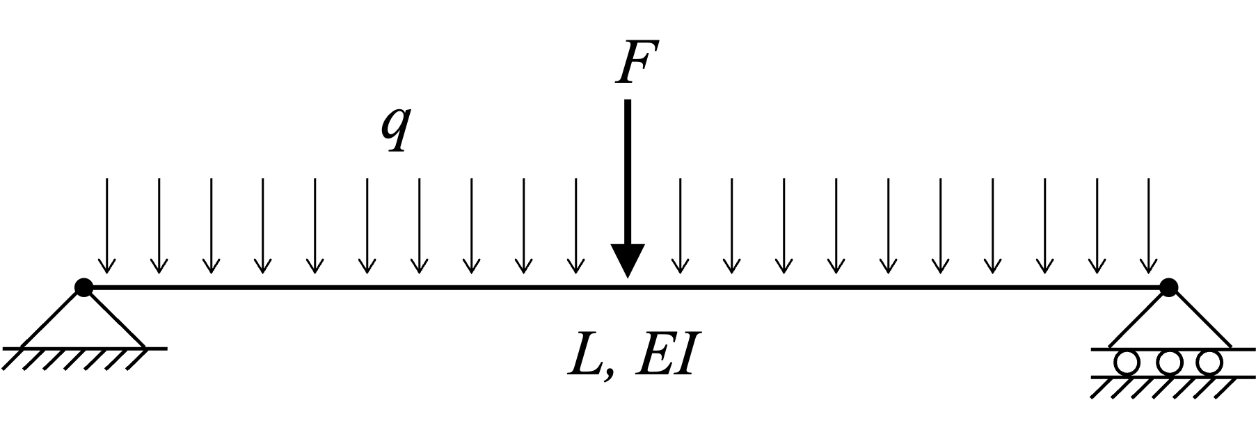
The random variables are \(E\), \(I\), \(q\), and \(F\), which serve as input to the following function that creates the structural model. Notice that the beam is split into two elements, with one node at midspan. This is done to place a point load there and to extract the bending moment at midspan from the analysis:
def createSimplySupportedInput(E, I, q, F):
    L = 8.0       # m
    A = 18774e-6  # m^2
    NODES = [[0.0, 0.0],
             [L/2, 0.0],
             [L,   0.0]]
    CONSTRAINTS = [[1, 1, 0],
                   [0, 0, 0],
                   [0, 1, 0]]
    ELEMENTS = [[5, E, A, I, q, 1, 2],
                [5, E, A, I, q, 2, 3]]
    LOADS = np.zeros((3, 3))
    LOADS[1, 1] = -F
    MASS = np.zeros((3, 3))
    SECTIONS = np.zeros(2)
    MATERIALS = np.zeros(2)
    return [NODES, CONSTRAINTS, ELEMENTS, SECTIONS, MATERIALS, LOADS, MASS]
Following the variable specification scheme established earlier in the book, here are the specs for the four input variables:
def simplySupportedVariableSpecs():
    E = 200e9         # N/m^2
    I = 462016882e-12 # m^4
    q = 20e3          # N/m
    F = 10e3          # N
    covE = 0.1
    covI = 0.05
    covq = 0.2
    covF = 0.2
    means = [E, I, q, F]
    stdvs = [covE*E, covI*I, covq*q, covF*F]
    distributions = ['Lognormal', 'Lognormal', 'Lognormal', 'Lognormal']
    correlation = []
    trackNode = 2
    trackDOF = 2
    DDMs = [['Element', 'E', [1, 2]],
            ['Element', 'I', [1, 2]],
            ['Element', 'q', [1, 2]],
            ['Nodal load', 2, 2]]
    return means, stdvs, distributions, correlation, trackNode, trackDOF, DDMs
The input to the structural model is here checked:
means, stdvs, distributions, correlation, trackNode, trackDOF, DDMs = simplySupportedVariableSpecs()
input = createSimplySupportedInput(*means)
checkModel(input)
All is well!The DSI is calculated here:
dsi = calculateDSI(input[0], input[1], input[2])The calculation gives DSI = 0.Here, the structural model is created and plotted:
structuralModel = model(input)
structuralModel.plotModel()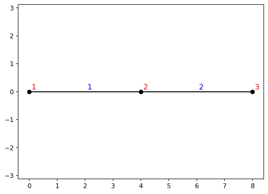
A linear static structural analysis is now run, without the adjoint method, because we seek several element responses. In the code below, element responses are extracted for the first element, i.e., the element on the left-hand side. That means M2 is the bending moment at midspan and V1 is the shear force at the left-hand side support in Figure 15.1:
u, dudx = linearStaticFirstOrderWithoutAdjoint(structuralModel, trackNode, trackDOF, DDMs)
void, void, void, void, elemlist = structuralModel.getData()
element = elemlist[0]
N, V1, V2, M1, M2 = element.getElementResponse()
dN, dV1, dV2, dM1, dM2 = element.getElementResponseSensitivity()
Second-moment response statistics for the displacement, \(u\), as well as M2 and V1 is calculated here:
covarianceMatrix = getCovMatrix(means, stdvs, correlation)
uStdv = np.sqrt(dudx.dot(covarianceMatrix.dot(dudx)))
print(f"The mean displacement is {u:.4f}m with {uStdv/np.abs(u)*100:.1f}% coefficient of variation")

M2stdv = np.sqrt(dM2.dot(covarianceMatrix.dot(dM2)))
print(f"The mean bending moment is {M2:.0f}Nm with {M2stdv/np.abs(M2)*100:.1f}% coefficient of variation")

V1stdv = np.sqrt(dV1.dot(covarianceMatrix.dot(dV1)))
print(f"The mean shear force is {V1:.0f}N with {V1stdv/np.abs(V1)*100:.1f}% coefficient of variation")
The mean displacement is -0.0127m with 21.4% coefficient of variation
The mean bending moment is -180000Nm with 17.9% coefficient of variation
The mean shear force is 85000N with 18.9% coefficient of variationThe negative bending moment at the right-hand side of the first element means counterclockwise moment, which in turn means tension at the bottom at midspan. The positive shear force at the left-hand side of the same element means clockwise, i.e., positive shear there. Correlation coefficients between the responses are also calculated:
covarianceMu = dM2.dot(covarianceMatrix.dot(dudx))
covarianceVu = dV1.dot(covarianceMatrix.dot(dudx))
covarianceMV = dM2.dot(covarianceMatrix.dot(dV1))

correlationMu = covarianceMu/(uStdv*M2stdv)
print(f"Correlation between u and M: {correlationMu:.2f}")

correlationVu = covarianceVu/(uStdv*V1stdv)
print(f"Correlation between u and V: {correlationVu:.2f}")

correlationMV = covarianceMV/(M2stdv*V1stdv)
print(f"Correlation between M and V: {correlationMV:.2f}")
Correlation between u and M: 0.85
Correlation between u and V: -0.85
Correlation between M and V: -1.00One limit-state function is defined for each of the three response quantities considered above. Here is the limit-state function for the displacement response, which accounts for the fact that the downwards displacement of the beam is negative:
def displacementLSF(x, threshold, needGradient=True):
    void, void, void, void, trackNode, trackDOF, DDMs = simplySupportedVariableSpecs()
    input = createSimplySupportedInput(*x)
    structuralModel = model(input)
    u, dudx = linearStaticFirstOrderWithoutAdjoint(structuralModel, trackNode, trackDOF, DDMs)
    return (threshold+u), dudx
Here is the limit-state function for the bending moment, accounting for the fact that the bending moment at the right-hand side of the first element is negative, meaning tension at the bottom:
def momentLSF(x, threshold, needGradient=True):
    void, void, void, void, trackNode, trackDOF, DDMs = simplySupportedVariableSpecs()
    input = createSimplySupportedInput(*x)
    structuralModel = model(input)
    u, dudx = linearStaticFirstOrderWithoutAdjoint(structuralModel, trackNode, trackDOF, DDMs)
    void, void, void, void, elemlist = structuralModel.getData()
    element = elemlist[0]
    N, V1, V2, M1, M2 = element.getElementResponse()
    dN, dV1, dV2, dM1, dM2 = element.getElementResponseSensitivity()
    return (threshold+M2), np.array(dM2)
Here is the limit-state function for the shear force:
def shearLSF(x, threshold, needGradient=True):
    void, void, void, void, trackNode, trackDOF, DDMs = simplySupportedVariableSpecs()
    input = createSimplySupportedInput(*x)
    structuralModel = model(input)
    u, dudx = linearStaticFirstOrderWithoutAdjoint(structuralModel, trackNode, trackDOF, DDMs)
    void, void, void, void, elemlist = structuralModel.getData()
    element = elemlist[0]
    N, V1, V2, M1, M2 = element.getElementResponse()
    dN, dV1, dV2, dM1, dM2 = element.getElementResponseSensitivity()
    return (threshold-V1), -np.array(dV1)
Three individual reliability analyses are now run, collecting \(\beta\) values and \(\mathbf{y}^*\) vectors on the way. As in Chapter 7, it is arbitrarily selected to set the exceedance threshold for each response to 1.8 times its first-order mean, for all responses:
betas = []
yStars = []
beta, xStar, yStar, kappa = iHLRFalgorithm(displacementLSF, 1.8*np.abs(u), means, stdvs, correlation, distributions, natafTransformation, False)
betas.append(beta)
yStars.append(yStar)
HLRF step 1: Check1=1.00e+00,Check2=0.00e+00, y-norm=1.000
HLRF step 2: Check1=5.87e-01,Check2=4.12e-02, y-norm=3.878
HLRF step 3: Check1=5.82e-02,Check2=6.52e-03, y-norm=2.915
HLRF step 4: Check1=7.73e-04,Check2=1.37e-03, y-norm=2.797
iHLRF algorithm converged with beta=2.797beta, xStar, yStar, kappa = iHLRFalgorithm(momentLSF, 1.8*np.abs(M2), means, stdvs, correlation, distributions, natafTransformation, False)
betas.append(beta)
yStars.append(yStar)HLRF step 1: Check1=1.00e+00,Check2=0.00e+00, y-norm=1.000
HLRF step 2: Check1=6.37e-01,Check2=6.87e-02, y-norm=4.710
HLRF step 3: Check1=6.79e-02,Check2=9.34e-03, y-norm=3.503
HLRF step 4: Check1=1.09e-03,Check2=2.41e-03, y-norm=3.342
iHLRF algorithm converged with beta=3.342beta, xStar, yStar, kappa = iHLRFalgorithm(shearLSF, 1.8*V1, means, stdvs, correlation, distributions, natafTransformation, False)
betas.append(beta)
yStars.append(yStar)HLRF step 1: Check1=1.00e+00,Check2=0.00e+00, y-norm=1.000
HLRF step 2: Check1=6.05e-01,Check2=3.51e-02, y-norm=4.475
HLRF step 3: Check1=6.19e-02,Check2=5.49e-03, y-norm=3.352
HLRF step 4: Check1=8.74e-04,Check2=1.04e-03, y-norm=3.209
iHLRF algorithm converged with beta=3.209The Ditlevsen bounds implemented in Chapter 7 are now evaluated for the series system consisting of all three limit-states analyzed above:
lower, upper, rhos = seriesSystemBounds(betas, yStars)Lower series system bound: 0.00270 (beta=2.782 from pf)
Upper series system bound: 0.00307 (beta=2.740 from pf)As in Chapter 7, we naturally observe that both bounds correspond to higher failure probability than the component problem with the highest failure probability, which is the displacement limit-state. Next, we examine the correlation between the limit-states:
counter = 0
for i in range(len(betas)):
    for j in range(i):
        print(f"G{j+1} - G{i+1} correlation: {rhos[counter]:.2f}")
        counter += 1
G1 - G2 correlation: 0.86
G1 - G3 correlation: 0.86
G2 - G3 correlation: 1.00We see that all correlation values are high, and nearly identical to those calculated earlier for the structural responses themselves. The minus sign in those earlier calculations stems from the fact that the displacement response and bending moment at the column base are negative.
15.3 Linear Portal Frame Revisited
The portal frame in Figure 1.2 served as demonstration example in the first half of this book. The same frame is re-analyzed here, but now it is parameterized to allow any number of elements in each of the two columns and the horizontal beam. That means the linear elastic frame is now discretized in the same manner as the distributed plasticity frame in Chapter 9:
def createLinearFrameRevisitedInput(varValues, L, H, I, A, nel):
    E =  varValues[:-2]
    q = varValues[-2]
    F = varValues[-1]
    NODES = []
    for i in range(nel+1):
        NODES.append([0.0, i*H/nel])
    for i in range(1, nel+1):
        NODES.append([i*L/nel, H])
    for i in range(1, nel+1):
        NODES.append([L, H-i*H/nel])
    CONSTRAINTS = np.zeros((3*nel+1, 3))
    CONSTRAINTS[0] = [1, 1, 1]
    CONSTRAINTS[3*nel] = [1, 1, 1]
    ELEMENTS = []
    for i in range(3*nel):
        if i < nel:
            ELEMENTS.append([5, E[i], A, I, q, i+1, i+2])
        else:
            ELEMENTS.append([5, E[i], A, I, 0, i+1, i+2])
    SECTIONS = np.zeros(3*nel)
    MATERIALS = np.zeros(3*nel)
    LOADS = np.zeros((3*nel+1, 3))
    LOADS[nel, 0] = F
    MASS = np.zeros((3*nel+1, 3))
    input = [NODES, CONSTRAINTS, ELEMENTS, SECTIONS, MATERIALS, LOADS, MASS]
    return input
The purpose of that discretization of the structural members is to have one stiffness variable per element, as seen in the variable specification shown below. There is one modulus of elasticity, \(E\), per element. The distributed load, \(q\), and the point load, \(F\), are the two additional variables:
def linearFrameRevisitedVariableSpecs(nel):
    E = 200e9   # N/m^2
    q = 20e3    # N/m
    F = 50e3    # N
    covE = 0.1
    covq = 0.2
    covF = 0.2
    stdvE = covE * E
    stdvq = covq * q
    stdvF = covF * F
    means = []
    stdvs = []
    DDMs = []
    for i in range(3*nel):
        means.append(E)
        stdvs.append(stdvE)
        DDMs.append(['Element', 'E', [i+1]])
    means.append(q)
    stdvs.append(stdvq)
    DDMs.append(['Element', 'q', range(1, nel+1)])
    means.append(F)
    stdvs.append(stdvF)
    DDMs.append(['Nodal load', nel+1, 1])
    correlation = []
    distributions = []
    trackNode = nel+1
    trackDOF = 1
    return means, stdvs, distributions, correlation, trackNode, trackDOF, DDMs
The height and width of the frame are not considered as random variables, neither are cross-section area and moment of inertia, whose values are given below, where the input is checked:
nel = 7
means, stdvs, distributions, correlation, trackNode, trackDOF, DDMs = linearFrameRevisitedVariableSpecs(nel)
H = 6             # m
L = 10            # m
A = 18774e-6      # m^2
I = 462016882e-12 # m^4
input = createLinearFrameRevisitedInput(means, L, H, I, A, nel)
checkModel(input)
All is well!Next, the DSI calculated in Chapter 1 is confirmed:
dsi = calculateDSI(input[0], input[1], input[2])The calculation gives DSI = 3.Next, the model is created and plotted:
structuralModel = model(input)
structuralModel.plotModel()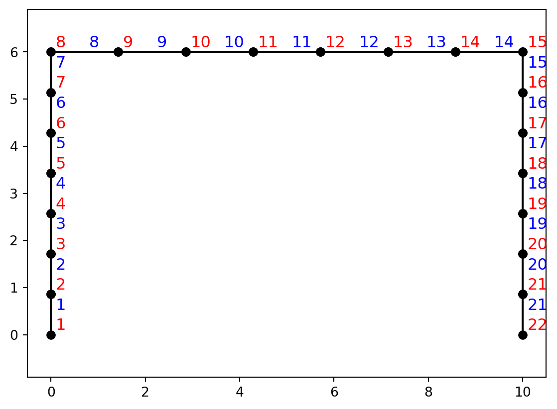
Here the linear static structural analysis is run with first-order sensitivities calculated by the adjoint method:
u, dudx = linearStaticFirstOrder(structuralModel, trackNode, trackDOF, DDMs)
print(f"Displacement: u={u:.4f}")
Displacement: u=0.0165We note that the displacement matches the value obtained in Chapter 3. It is checked offline that the same goes for the sensitivity of that displacement to \(q\) and \(F\). However, attention is here given to the sensitivities \(\frac{\partial u}{\partial E_i}\). The importance ranking technique from Section 3.4.4 is utilized to rank the importance of the stiffness of each element:
importanceVector = dudx*stdvs
sortedVector = np.flip(np.argsort(np.abs(importanceVector)))
rank = 1
for i in sortedVector[2:]:
    print(f"{rank:2}. Element {DDMs[i][2][0]}"); rank+=1
1. Element 1
2. Element 21
3. Element 14
4. Element 2
5. Element 8
6. Element 20
7. Element 7
8. Element 15
9. Element 13
10. Element 9
11. Element 19
12. Element 6
13. Element 3
14. Element 16
15. Element 12
16. Element 10
17. Element 18
18. Element 5
19. Element 11
20. Element 17
21. Element 4It is unsurprising that Elements 1 and 21 are most important; they are the elements at the fixed base of both columns. The adjacent elements are also important, especially on the left-hand side where we know the bending moment is greater. Elements adjacent to the upper corners of the frame also appear high in the importance ranking. It makes sense that the stiffness there is influential on the displacement response, because the bending moments are large there, albeit less than at the base of the columns.
15.4 Vertical Dynamic Truss
A pure truss is here modelled. It is parameterized such that one braced “panel” is stacked on top of the next, with the number of panels given by nStorys. The nonlinear truss element from Chapter 8 is employed for all members. Also notice that all nodes away from the base of the structure is given a lumped mass:
def createVerticalTrussInput(varValues, L, H, A, fy, alpha, nStorys):
    nel = 5*nStorys
    E =  varValues[:nel]
    M = varValues[nel:]
    NODES = []
    for i in range(nStorys+1):
        NODES.append([0, i*H])
        NODES.append([L, i*H])
    CONSTRAINTS = [[1, 1],
                   [1, 1]]
    for i in range(nStorys):
        CONSTRAINTS.append([0, 0])
        CONSTRAINTS.append([0, 0])
    elementType = 2
    N0 = 0.0
    ELEMENTS = []
    for i in range(nStorys):
        ELEMENTS.append([elementType, N0, 2*i+1, 2*i+3])
        ELEMENTS.append([elementType, N0, 2*i+2, 2*i+4])
        ELEMENTS.append([elementType, N0, 2*i+1, 2*i+4])
        ELEMENTS.append([elementType, N0, 2*i+2, 2*i+3])
        ELEMENTS.append([elementType, N0, 2*i+3, 2*i+4])
    SECTIONS = []
    for i in range(nel):
        SECTIONS.append(['Truss', A])
    MATERIALS = []
    for i in range(nel):
        MATERIALS.append(['Bilinear', E[i], fy, alpha])
    LOADS = np.zeros(((nStorys+1)*2, 2))
    MASS = [[0, 0],
            [0, 0]]
    for i in range(nStorys):
        MASS.append([M[i], 0])
        MASS.append([M[i+1], 0])
    return [NODES, CONSTRAINTS, ELEMENTS, SECTIONS, MATERIALS, LOADS, MASS]
There is one modulus of elasticity, \(E\), in each element. Similarly, all the lumped masses, \(M\), are different variables. That is specified below, together with rather high mass values, in order to see some yielding in the subsequent nonlinear analysis with the El Centro ground motion:
def verticalTrussVariableSpecs(nStorys):
    E = 200e9     # N/m^2
    M = 4e3       # kg
    covE = 0.1
    covM = 0.2
    stdvE = covE * E
    stdvM = covM * M
    means = []
    stdvs = []
    DDMs = []
    nel = 5*nStorys
    for i in range(nel):
        means.append(E)
        stdvs.append(stdvE)
        DDMs.append(['Element', 'E', [i+1]])
    for i in range(nStorys):
        means.append(M)
        means.append(M)
        stdvs.append(stdvM)
        stdvs.append(stdvM)
        node = 2*(i+1)
        dM = np.zeros(((nStorys+1)*2, 2))
        dM[node, 0] = 1
        DDMs.append(['Node', 'M', dM])
        node = 2*(i+1)+1
        dM = np.zeros(((nStorys+1)*2, 2))
        dM[node, 0] = 1
        DDMs.append(['Node', 'M', dM])
    correlation = []
    distributions = []
    trackNode = [2+2*nStorys]
    trackDOF = [1]
    return means, stdvs, distributions, correlation, trackNode, trackDOF, DDMs
Next, the input to the structural model is generated and checked. Notice that a low yield stress is provided to get some yielding in the subsequent nonlinear analysis:
nStorys = 5
means, stdvs, distributions, correlation, trackNode, trackDOF, DDMs = verticalTrussVariableSpecs(nStorys)
L = 3
H = 3
A = 0.0025
fy = 200e6
alpha = 0.05
input = createVerticalTrussInput(means, L, H, A, fy, alpha, nStorys)
checkModel(input)
All is well!The DSI is calculated here:
dsi = calculateDSI(input[0], input[1], input[2])The calculation gives DSI = 5.The model is created and plotted here:
structuralModel = model(input)
structuralModel.plotModel()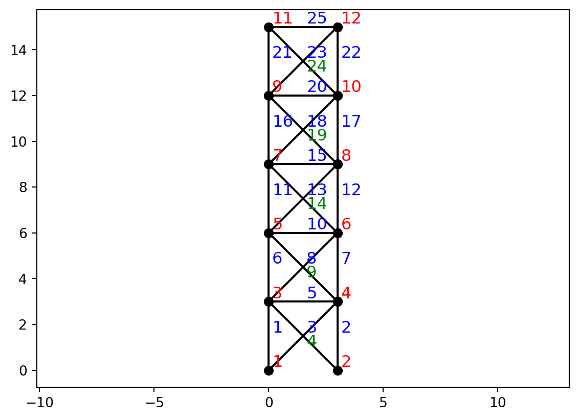
The natural frequencies are calculated here:
gammas, phi = structuralModel.getNaturalFrequencies()Found 10 natural frequencies:
Natural frequency number 1 is 11.4 rad/sec. (period=0.5510 sec.)
Natural frequency number 2 is 58.0 rad/sec. (period=0.1083 sec.)
Natural frequency number 3 is 127.1 rad/sec. (period=0.0494 sec.)
Natural frequency number 4 is 188.0 rad/sec. (period=0.0334 sec.)
Natural frequency number 5 is 228.6 rad/sec. (period=0.0275 sec.)
Natural frequency number 6 is 290.2 rad/sec. (period=0.0217 sec.)
Natural frequency number 7 is 301.4 rad/sec. (period=0.0208 sec.)
Natural frequency number 8 is 319.4 rad/sec. (period=0.0197 sec.)
Natural frequency number 9 is 337.9 rad/sec. (period=0.0186 sec.)
Natural frequency number 10 is 351.3 rad/sec. (period=0.0179 sec.)Next, the El Centro ground motion is loaded:
dt = 0.02
gmMatrix = readGroundMotion("ElCentro.txt", dt)
Both a linear and a nonlinear dynamic analysis are run, with the response from the linear analysis shown as a dashed line and yielding in the nonlinear analysis marked with a red line:
targetDamping = 0.05
dampingModel = ['Modal', 'Initial', targetDamping]
uLin, dudxLin = linearDynamicAnalysis(structuralModel, 'Modal', targetDamping, gmMatrix, trackNode[0], trackDOF[0], DDMs)
t, gm, u, v, a, dudx, dvdx, dadx, dnl1, dnl2 = nonlinearDynamicAnalysis(structuralModel, dampingModel, gmMatrix, trackNode, trackDOF, 1, [])
plt.figure()
plt.plot(t, uLin, 'k--', linewidth=1.0)
for i in range(1, len(t)):
    if dnl1[i] > 1:
        plt.plot([t[i-1], t[i]], [u[0, i-1], u[0, i]], 'r-', linewidth=1.0)
    else:
        plt.plot([t[i-1], t[i]], [u[0, i-1], u[0, i]], 'k-', linewidth=1.0)
plt.xlabel("Time [sec.]")
plt.grid(True)
plt.show()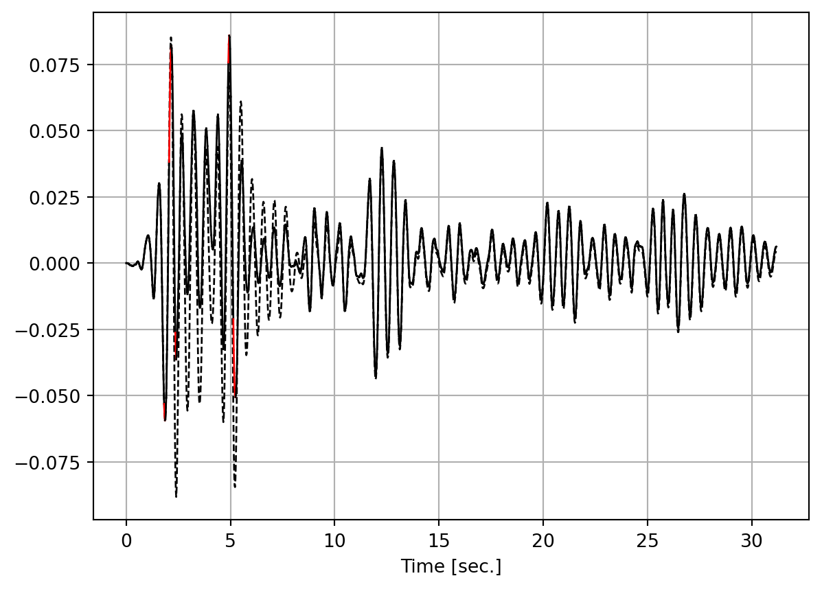
The response sensitivity with respect to stiffnesses, from the linear analysis, are plotted here, with stiffness numbers corresponding to the element numbers in the truss plotted earlier:
nel = 5*nStorys
timeWindow = range(int(0.12*len(t)), int(0.18*len(t)))
colourNames = ['red', 'lawngreen', 'yellowgreen', 'aqua', 'magenta', 'black', 'blue', 'blueviolet', 'chocolate', 'yellow', 'cyan', 'darkblue', 'darkgray', 'darkorange', 'darkseagreen', 'darkslateblue', 'deeppink', 'gold', 'gray', 'green', 'lightblue', 'lightgreen', 'lightpink', 'orange', 'slateblue']
plt.figure()
for i in range(nel):
    plt.plot(t[timeWindow], dudxLin[i, timeWindow], color=colourNames[i], linestyle='solid', linewidth=1.0, label=(f"E{i+1}"))
plt.xlabel("Time [sec.]")
plt.grid(True)
plt.legend(loc='upper right')
plt.show()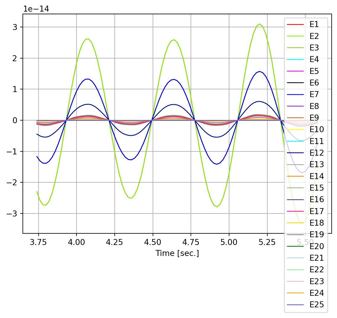
It is perhaps not surprising that the stiffness in Elements 2, 7, and 12 appear most important; they are stacked on top of each other on the right-hand side of the truss, as seen from the earlier plot. This means they are the important elements to carry the inertia forces into the support.
The response sensitivity with respect to mass, from the linear analysis, are plotted next, with mass numbers corresponding to the node numbers in plot of the truss:
plt.figure()
for i in range(nel, len(dudxLin)):
    plt.plot(t[timeWindow], dudxLin[i, timeWindow], color=colourNames[i-nel], linestyle='solid', linewidth=1.0, label=(f"M{i+3-nel}"))
plt.xlabel("Time [sec.]")
plt.grid(True)
plt.legend(loc='upper right')
plt.show()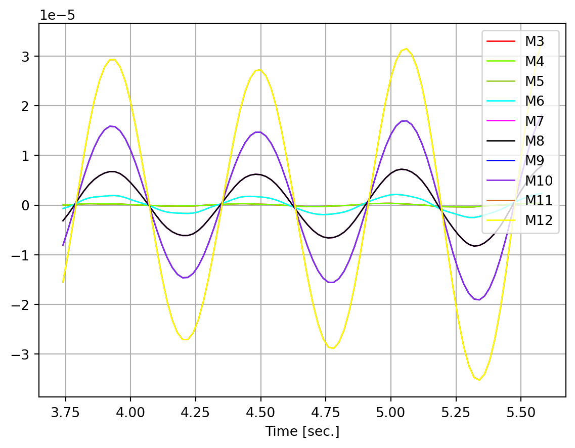
We see that one of the lumped masses at the very top right-hand side of the truss structure, i.e., Node 12 is the most influential mass. It is also interesting to see that the vibrations are such that the masses immediately below that top mass, i.e., mass at Nodes 10, 8, and 6 follow thereafter in importance.
15.5 Horizontal Static Truss
A truss structure parameterized in a manner similar to the one in the previous section is here analyzed. However, it is laid down horizontally, essentially acting as a bridge between a pinned support on the left and and a roller support on the right. Furthermore, the analysis considered now is static instead of dynamic. What was referred to as nStorys in the previous section is now called nSegments:
def createHorizontalTrussInput(varValues, L, H, A, alpha, nSegments):
    nel = 5*nSegments+1
    E =  varValues[:nel]
    fy = varValues[nel:(2*nel)]
    F = varValues[(2*nel):]
    NODES = []
    for i in range(nSegments+1):
        NODES.append([i*L, 0])
        NODES.append([i*L, H])
    CONSTRAINTS = np.zeros(((nSegments+1)*2, 2))
    CONSTRAINTS[0] = [1, 1]
    CONSTRAINTS[-2] = [0, 1]
    elementType = 2
    N0 = 0.0
    ELEMENTS = [[elementType, N0, 1, 2]]
    for i in range(nSegments):
        ELEMENTS.append([elementType, N0, 2*i+1, 2*i+3])
        ELEMENTS.append([elementType, N0, 2*i+2, 2*i+4])
        ELEMENTS.append([elementType, N0, 2*i+1, 2*i+4])
        ELEMENTS.append([elementType, N0, 2*i+2, 2*i+3])
        ELEMENTS.append([elementType, N0, 2*i+3, 2*i+4])
    SECTIONS = []
    for i in range(nel):
        SECTIONS.append(['Truss', A])
    MATERIALS = []
    for i in range(nel):
        MATERIALS.append(['Bilinear', E[i], fy[i], alpha])
    LOADS = np.zeros(((nSegments+1)*2, 2))
    for i in range(nSegments-1):
        LOADS[2*i+2, 1] = -F[i]
    MASS = np.zeros(((nSegments+1)*2, 2))
    return [NODES, CONSTRAINTS, ELEMENTS, SECTIONS, MATERIALS, LOADS, MASS]
There is one stiffness and one yield stress variable in each element. Also, the point loads at all free lower nodes of the truss are individual random variables:
def horizontalTrussVariableSpecs(nSegments):
    E = 200e9     # N/m^2
    fy = 350e6    # N/m^2
    F = 180e3     # N
    covE = 0.1
    covfy = 0.2
    covF = 0.2
    stdvE = covE * E
    stdvfy = covfy * fy
    stdvF = covF * F
    means = []
    stdvs = []
    DDMs = []
    distributions = []
    nel = 5*nSegments+1
    for i in range(nel):
        means.append(E)
        stdvs.append(stdvE)
        DDMs.append(['Element', 'E', [i+1]])
        distributions.append('Lognormal')
    for i in range(nel):
        means.append(fy)
        stdvs.append(stdvfy)
        DDMs.append(['Element', 'fy', [i+1]])
        distributions.append('Lognormal')
    for i in range(nSegments-1):
        means.append(F)
        stdvs.append(stdvF)
        DDMs.append(['Nodal load', 2*i+3, 2])
        distributions.append('Lognormal')
    correlation = []
    if nSegments % 2 == 0:
        trackNode = int((2*nSegments+2)/2)
    else:
        trackNode = int((2*nSegments+1)/2)
    trackDOF = 2
    return means, stdvs, distributions, correlation, trackNode, trackDOF, DDMs
The input is here created and checked:
nSegments = 6
means, stdvs, distributions, correlation, trackNode, trackDOF, DDMs = horizontalTrussVariableSpecs(nSegments)
L = 3
H = 3
A = 0.002
alpha = 0.05
input = createHorizontalTrussInput(means, L, H, A, alpha, nSegments)
checkModel(input)
All is well!The DSI is calculated here:
dsi = calculateDSI(input[0], input[1], input[2])The calculation gives DSI = 6.Next, the structural model is created and plotted:
structuralModel = model(input)
structuralModel.plotModel()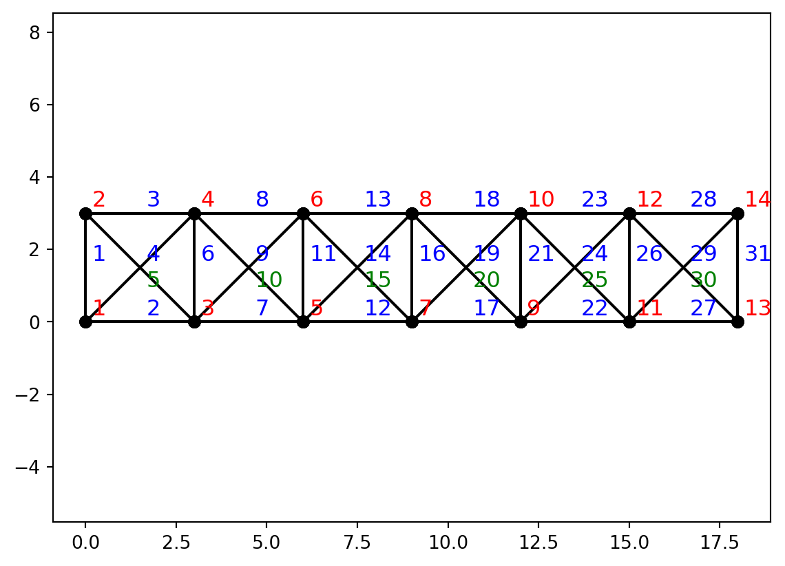
Taking advantage of the capabilities of Element 2, i.e., the nonlinear truss element, a nonlinear static analysis is now conducted:
nsteps = 20
dt = 0.05
t, lamda, u, dudx, Hessian = nonlinearStaticAnalysis(structuralModel, nsteps, dt, trackNode, trackDOF, DDMs, 1)
plt.figure()
plt.plot(u, lamda, 'ko-')
plt.grid(True)
plt.xlabel("Displacement [m]")
plt.ylabel("Load factor")
plt.show()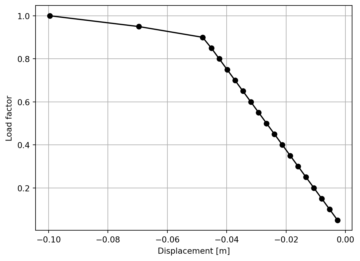
The resulting load-displacement curve, shown above, reflects that the downwards displacement is negative. It also reveals that yielding takes place in the last few load increments. The response that is plotted is the vertical displacement at the node at midspan, or nearest the midspan when the number of segments is an odd number.
The importance ranking technique used earlier in this chapter for the linear frame is now repeated here. For brevity, only the fifteen most important variables are printed:
names = []
nel = 5*nSegments+1
for i in range(nel):
    names.append(f'E{i+1}')
for i in range(nel):
    names.append(f'fy{i+1}')
for i in range(nSegments-1):
    names.append(f'F{i+1}')
importanceVector = dudx[:,-1]*stdvs
sortedVector = np.flip(np.argsort(np.abs(importanceVector)))
rank = 1
for i in sortedVector[:15]:
    print(f"{rank:2}. Element {names[i]}"); rank+=1
1. Element F3
2. Element F2
3. Element F4
4. Element fy13
5. Element fy18
6. Element fy12
7. Element fy17
8. Element F1
9. Element F5
10. Element E13
11. Element E18
12. Element E12
13. Element E17
14. Element E8
15. Element E23As often is the case, loads appear at the top of the importance ranking. In this case, the three point loads nearest the midspan of the truss are the most important variables. The list printed above also shows that the yield stress in the chord members closest to midspan are the four most important variables after the loads. The stiffness of those chord members also appear in the top-15. The element numbers are given in the earlier plot of the truss.
Next, reliability analyses are carried out, with the first- and second-order reliability methods. Encompassing many of the specifications given above, and accounting for the fact that the displacement response is negative, the limit-state function is defined as follows:
def nonlinearHorizontalTrussLSF(x, threshold, needGradient=True):
    nSegments = 6
    void, void, void, void, trackNode, trackDOF, DDMs = horizontalTrussVariableSpecs(nSegments)
    L = 3
    H = 3
    A = 0.002
    alpha = 0.05
    input = createHorizontalTrussInput(x, L, H, A, alpha, nSegments)
    structuralModel = model(input)
    nsteps = 20
    dt = 0.05
    t, lamda, u, dudx, Hessian = nonlinearStaticAnalysis(structuralModel, nsteps, dt, trackNode, trackDOF, DDMs, 1)
    return (threshold+u[-1]), dudx[:, -1]
Using the load-displacement curve given above as a guide, a first-order reliability analysis is carried out for the displacement response threshold 0.4m:
threshold = 0.4
beta, xStar, yStar, kappa = iHLRFalgorithm(nonlinearHorizontalTrussLSF, threshold, means, stdvs, correlation, distributions, natafTransformation, False, True)
HLRF step 1: Check1=1.00e+00,Check2=0.00e+00, y-norm=1.000
HLRF step 2: Check1=1.54e-01,Check2=4.49e-01, y-norm=4.093
HLRF step 3: Check1=2.47e-02,Check2=7.14e-02, y-norm=3.261
HLRF step 4: Check1=4.94e-04,Check2=9.63e-03, y-norm=3.315
iHLRF algorithm converged with beta=3.315We see that the iHLRF algorithm converges in this case, without the golden section search for optimal step sizes. Next, a second-order reliability analysis is conducted, using the design point from the iHLRF algorithm as input:
input = createHorizontalTrussInput(xStar, L, H, A, alpha, nSegments)
structuralModel = model(input)
t, lamda, u, dudx, xHessian = nonlinearStaticAnalysis(structuralModel, nsteps, dt, trackNode, trackDOF, DDMs, 2)
pfFORM, pfSORM, curvatures = SORM(beta, xStar, yStar, dudx[:,-1], xHessian[:,:,-1], means, stdvs, correlation, distributions)
FORM failure probability: 0.00046 (Reliability index 3.315)
SORM failure probability: 0.00045 (Reliability index 3.322, from pf)That SORM estimate of the reliability is slightly higher than the first-order estimate.
Next, a linear structural analysis is conducted. It is inappropriate to employ a linear analysis algorithm because the nonlinear truss element has features related to increments and history variables that are not handled by linear analysis algorithms. Therefore, the analysis above is repeated, but now only up to 80% of the load applied earlier. That means no yielding, i.e., a linear analysis. Because of the history variables stored in the elements of the structural model, we must now re-create that model to refresh it:
nsteps = 16 # Gives maximum load factor 0.8 for the given delta-t
dt = 0.05
input = createHorizontalTrussInput(means, L, H, A, alpha, nSegments)
structuralModel = model(input)
t, lamda, u, dudx, Hessian = nonlinearStaticAnalysis(structuralModel, nsteps, dt, trackNode, trackDOF, DDMs, 1)
plt.figure()
plt.plot(u, lamda, 'ko-')
plt.grid(True)
plt.xlabel("Displacement [m]")
plt.ylabel("Load factor")
plt.show()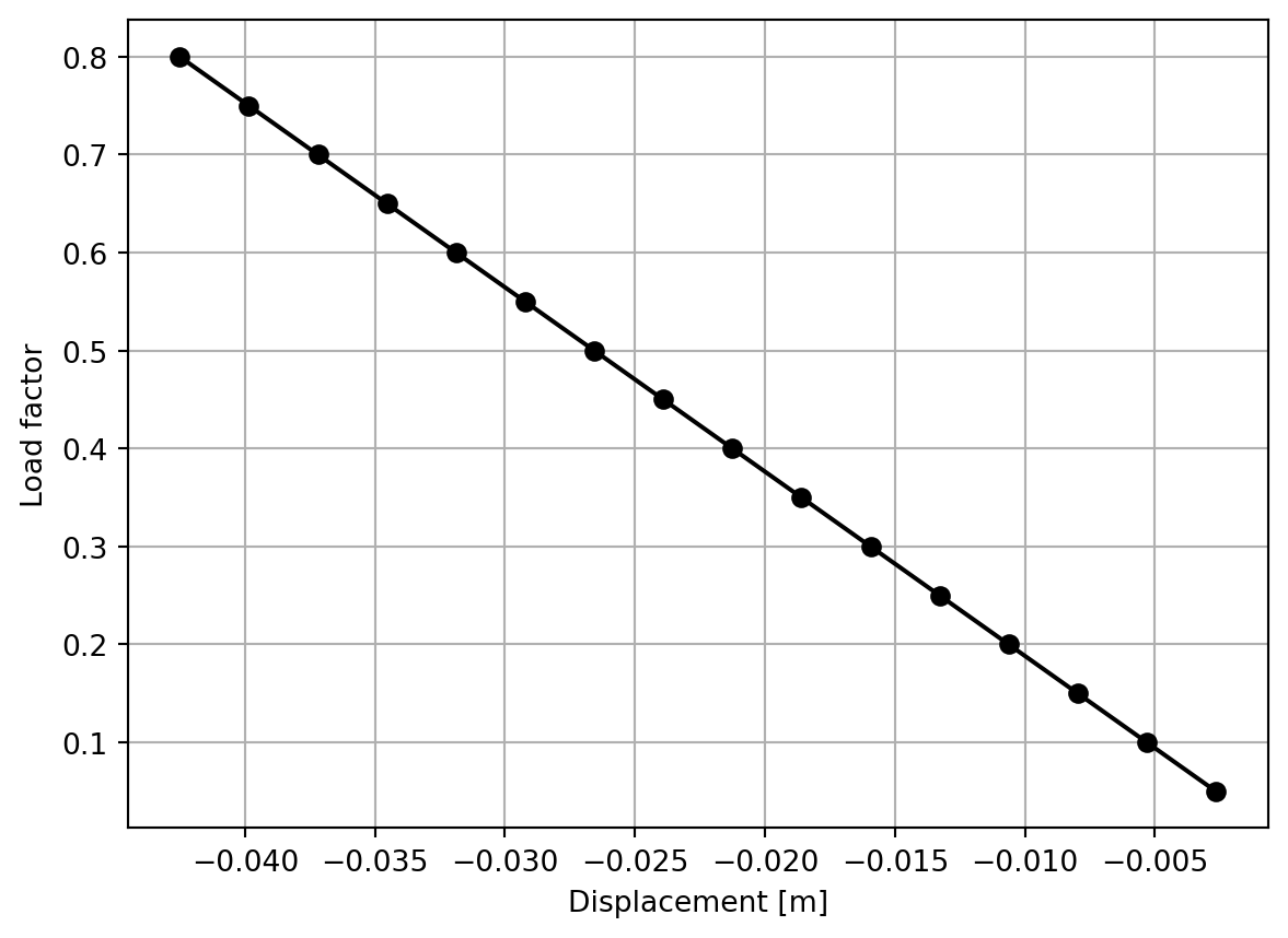
The resulting load-displacement curve confirms the linearity of the response. As a reference for another linear analysis in the next section, the final displacement is here printed:
print(f"Displacement after the last load increment: {u[-1]:.5f}m")Displacement after the last load increment: -0.04251mThe importance ranking for the linear case is printed here:
importanceVector = dudx[:,-1]*stdvs
sortedVector = np.flip(np.argsort(np.abs(importanceVector)))
rank = 1
for i in sortedVector[:15]:
    print(f"{rank:2}. Element {names[i]}"); rank+=1
1. Element F3
2. Element F2
3. Element F4
4. Element F5
5. Element F1
6. Element E13
7. Element E18
8. Element E12
9. Element E17
10. Element E23
11. Element E8
12. Element E7
13. Element E22
14. Element E30
15. Element E4We now see that all five loads are at the top of the importance ranking. Naturally, the yield stress variables have disappeared from the list because this is now a linear analysis. Looking at the previous ranking, for the nonlinear analysis, it is predictable that the stiffness of the chord members at the middle of the truss are now the variables that follow behind the loads in having the highest influence on the displacement response.
Reliability analysis is not conducted here, at the 80% load level, because the structure will enter the nonlinear response range before a reasonably high response threshold is reached, essentially duplicating the reliability analysis conducted above.
15.6 Horizontal Truss Revisited
The axial force in each member of the horizontal truss is now examined. Utilizing capabilities introduced in Chapter 7, the objective is to conduct a system reliability analysis with limit-states defined by those forces. However, the linear structural analysis algorithm developed in Chapter 7 does not fit the nonlinear truss element utilized in the previous section. For that reason, a linear truss element is implemented here. It stores its axial force and corresponding sensitivities in the same way that the linear frame element did for its interenal forces in Chapter 7. The linear truss element is labelled Element 1:
class element1():

    def __init__(self, E, A, elno):
        self.no = elno
        self.E  = E
        self.A  = A
        self.N = 0
        self.dN = np.array([])

    def initialize(self, xyz):
        dx = xyz[1,:] - xyz[0,:]
        self.L = np.sqrt(dx.dot(dx))
        dx = dx / self.L
        self.Tbg = np.array([-dx[0], -dx[1], dx[0], dx[1]])

    def stateDetermination(self, xyz, ugMatrix, theLambda):
        ug = ugMatrix[:, 0]
        ub = self.Tbg.dot(ug)
        EA = self.E * self.A
        Kb = EA / self.L
        Fb = Kb * ub
        Fg_tilde = self.Tbg.dot(Fb)
        Kg = np.outer(self.Tbg.dot(Kb), self.Tbg)
        return Fg_tilde, Kg

    def stateDerivative(self, xyz, ugMatrix, theLambda, ddmParameter, ddmIndex=0, ddmIsHere=False, dkflag='none'):
        ug = ugMatrix[:, 0]
        ub = self.Tbg.dot(ug)
        if ddmParameter == 'E' and ddmIsHere:
            dEA = self.A
        elif ddmParameter == 'A' and ddmIsHere:
            dEA = self.E
        else:
            dEA = 0.0
        dKb = dEA / self.L
        dFb = dKb * ub
        dFg_tilde = self.Tbg.dot(dFb)
        dKg = np.outer(self.Tbg.dot(dKb), self.Tbg)
        return dFg_tilde, dKg, 0

    def setElementResponse(self, ugMatrix, theLambda):
        ug = ugMatrix[:, 0]
        ub = self.Tbg.dot(ug)
        Kb = self.E * self.A / self.L
        self.N = Kb * ub

    def setElementResponseSensitivity(self, ugMatrix, dug, theLambda, ddmParameter, ddmIsHere):
        ug = ugMatrix[:, 0]
        ub = self.Tbg.dot(ug)
        dub = self.Tbg.dot(dug)
        EA = self.E * self.A
        Kb = EA / self.L
        if ddmParameter == 'E' and ddmIsHere:
            dEA = self.A
        elif ddmParameter == 'A' and ddmIsHere:
            dEA = self.E
        else:
            dEA = 0.0
        dKb = dEA / self.L
        self.dN = np.append(self.dN, dKb*ub + Kb*dub)

    def getElementResponse(self):
        return self.N

    def getElementResponseSensitivity(self):
        return self.dN
The structural model class is amended, as has been done earlier in this book, to facilitate the creation of instances of Element 1:
class model(model):
    def createElements(self):
        nelem = len(self.ELEMENTS)
        ellist = []
        for i in range(nelem):
            eltyp = self.ELEMENTS[i][0]
            if eltyp == 1:
                E = self.ELEMENTS[i][1]
                A = self.ELEMENTS[i][2]
                el = element1(E, A, i+1)
            elif eltyp == 2:
                N0 = self.ELEMENTS[i][1]
                el = element2(N0, self.SECTIONS[i], self.MATERIALS[i], i+1)
            elif eltyp == 5:
                E = self.ELEMENTS[i][1]
                A = self.ELEMENTS[i][2]
                I = self.ELEMENTS[i][3]
                q = self.ELEMENTS[i][4]
                el = element5(E, A, I, q, i+1)
            elif eltyp == 12:
                nsec = self.ELEMENTS[i][1]
                q = self.ELEMENTS[i][2]
                el = element12(nsec, q, self.SECTIONS[i], self.MATERIALS[i], i+1)
            ellist.append(el)
        return ellist
The function that creates the horizontal truss is slightly modified, compared to the previous section, to make use of the new linear truss element:
def createHorizontalTrussRevisitedInput(F, L, H, E, A, nSegments):
    NODES = []
    for i in range(nSegments+1):
        NODES.append([i*L, 0])
        NODES.append([i*L, H])
    CONSTRAINTS = np.zeros(((nSegments+1)*2, 2))
    CONSTRAINTS[0] = [1, 1]
    CONSTRAINTS[-2] = [0, 1]
    elementType = 1
    elementCount = 0
    ELEMENTS = [[elementType, E, A, 1, 2]]
    for i in range(nSegments):
        ELEMENTS.append([elementType, E, A, 2*i+1, 2*i+3]); elementCount+=1
        ELEMENTS.append([elementType, E, A, 2*i+2, 2*i+4]); elementCount+=1
        ELEMENTS.append([elementType, E, A, 2*i+1, 2*i+4]); elementCount+=1
        ELEMENTS.append([elementType, E, A, 2*i+2, 2*i+3]); elementCount+=1
        ELEMENTS.append([elementType, E, A, 2*i+3, 2*i+4]); elementCount+=1
    SECTIONS = np.zeros(len(ELEMENTS))
    MATERIALS = np.zeros(len(ELEMENTS))
    LOADS = np.zeros(((nSegments+1)*2, 2))
    for i in range(nSegments-1):
        LOADS[2*i+2, 1] = -F[i]
    MASS = np.zeros(((nSegments+1)*2, 2))
    return [NODES, CONSTRAINTS, ELEMENTS, SECTIONS, MATERIALS, LOADS, MASS]
The variable specifications are also altered, to remove the yield stress and to maintain the 80% load applied in the linear analysis in the previous section. Furthermore, the modulus of elasticity for each element is no longer a random variable here. That is because member stiffness values have little influence on the internal forces of a structure; in fact, for statically determinate structures that influence is zero. That means the loads are kept as the only random variables in this example:
def horizontalTrussRevisitedVariableSpecs(nSegments):
    F = 180e3*0.8  # N
    covF = 0.2
    stdvF = covF * F
    means = []
    stdvs = []
    DDMs = []
    for i in range(nSegments-1):
        means.append(F)
        stdvs.append(stdvF)
        DDMs.append(['Nodal load', 2*i+3, 2])
    correlation = []
    distributions = []
    if nSegments % 2 == 0:
        trackNode = int((2*nSegments+2)/2)
    else:
        trackNode = int((2*nSegments+1)/2)
    trackDOF = 2
    return means, stdvs, distributions, correlation, trackNode, trackDOF, DDMs
Next, the structural model is created and the truss is plotted in order to have the element numbers handy:
nSegments = 6
means, stdvs, distributions, correlation, trackNode, trackDOF, DDMs = horizontalTrussRevisitedVariableSpecs(nSegments)
L = 3
H = 3
E = 200e9
A = 0.002
input = createHorizontalTrussRevisitedInput(means, L, H, E, A, nSegments)
structuralModel = model(input)
structuralModel.plotModel()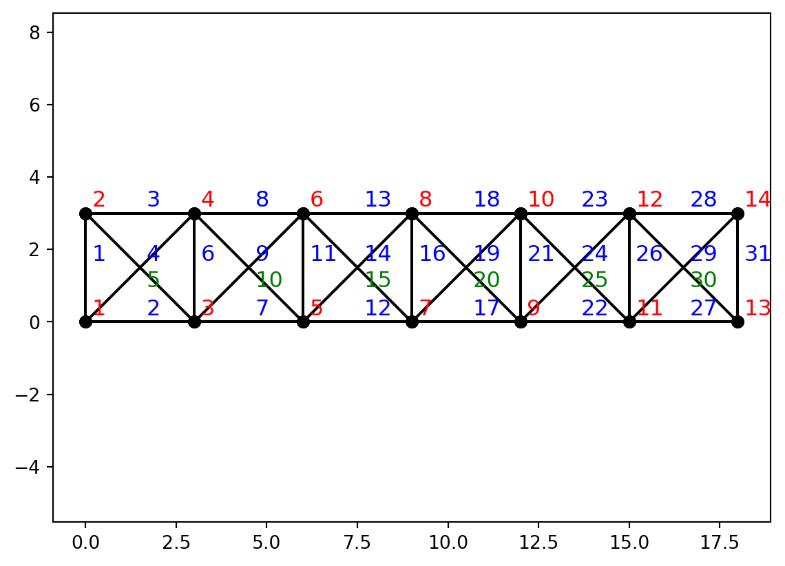
That truss is now analyzed, with the linear static structural analysis algorithm from Chapter 7. The displacement response is printed for comparison with the result obtained in the linear analysis near the end of the previous section:
u, dudx = linearStaticFirstOrderWithoutAdjoint(structuralModel, trackNode, trackDOF, DDMs)
print(f"Displacement: {u:.5f}m")
Displacement: -0.04251mAs expected, the displacement matches that from the linear analysis in the previous section. Next, we print the axial force in all elements of the truss:
void, void, void, void, elemlist = structuralModel.getData()
for i in range(len(elemlist)):
    N = elemlist[i].getElementResponse()
    print(f"N[{i+1}] = {N*1e-3:6.1f}kN")
N[1] = -167.3kN
N[2] = 192.7kN
N[3] = -167.3kN
N[4] = -272.6kN
N[5] = 236.5kN
N[6] = 69.8kN
N[7] = 453.0kN
N[8] = -483.0kN
N[9] = -131.6kN
N[10] = 173.9kN
N[11] = 44.9kN
N[12] = 599.9kN
N[13] = -624.1kN
N[14] = -33.8kN
N[15] = 68.0kN
N[16] = 47.8kN
N[17] = 599.9kN
N[18] = -624.1kN
N[19] = 68.0kN
N[20] = -33.8kN
N[21] = 44.9kN
N[22] = 453.0kN
N[23] = -483.0kN
N[24] = 173.9kN
N[25] = -131.6kN
N[26] = 69.8kN
N[27] = 192.7kN
N[28] = -167.3kN
N[29] = 236.5kN
N[30] = -272.6kN
N[31] = -167.3kNBecause of the importance ranking in the previous section, it is unsurprising that Elements 12, 13, 17, and 18 have the hightest axial forces. That is why limit-state functions are defined below for those four axial forces. For completeness, it would be better to define one limit-state function for every single member of the truss. However, that is omitted here for brevity, focusing on Elements 12, 13, 17, and 18:
def element12LSF(x, threshold, needGradient=True):
    nSegments = 6
    void, void, void, void, trackNode, trackDOF, DDMs = horizontalTrussRevisitedVariableSpecs(nSegments)
    L = 3
    H = 3
    E = 200e9
    A = 0.002
    input = createHorizontalTrussRevisitedInput(x, L, H, E, A, nSegments)
    structuralModel = model(input)
    void, void = linearStaticFirstOrderWithoutAdjoint(structuralModel, trackNode, trackDOF, DDMs)
    void, void, void, void, elemlist = structuralModel.getData()
    theElement = elemlist[11]
    N = theElement.getElementResponse()
    dN = theElement.getElementResponseSensitivity()
    return (threshold-N), -np.array(dN) # Note: Axial force is positive

def element13LSF(x, threshold, needGradient=True):
    nSegments = 6
    void, void, void, void, trackNode, trackDOF, DDMs = horizontalTrussRevisitedVariableSpecs(nSegments)
    L = 3
    H = 3
    E = 200e9
    A = 0.002
    input = createHorizontalTrussRevisitedInput(x, L, H, E, A, nSegments)
    structuralModel = model(input)
    void, void = linearStaticFirstOrderWithoutAdjoint(structuralModel, trackNode, trackDOF, DDMs)
    void, void, void, void, elemlist = structuralModel.getData()
    theElement = elemlist[12]
    N = theElement.getElementResponse()
    dN = theElement.getElementResponseSensitivity()
    return (threshold+N), np.array(dN) # Note: Axial force is negative

def element17LSF(x, threshold, needGradient=True):
    nSegments = 6
    void, void, void, void, trackNode, trackDOF, DDMs = horizontalTrussRevisitedVariableSpecs(nSegments)
    L = 3
    H = 3
    E = 200e9
    A = 0.002
    input = createHorizontalTrussRevisitedInput(x, L, H, E, A, nSegments)
    structuralModel = model(input)
    void, void = linearStaticFirstOrderWithoutAdjoint(structuralModel, trackNode, trackDOF, DDMs)
    void, void, void, void, elemlist = structuralModel.getData()
    theElement = elemlist[16]
    N = theElement.getElementResponse()
    dN = theElement.getElementResponseSensitivity()
    return (threshold-N), -np.array(dN) # Note: Axial force is positive

def element18LSF(x, threshold, needGradient=True):
    nSegments = 6
    void, void, void, void, trackNode, trackDOF, DDMs = horizontalTrussRevisitedVariableSpecs(nSegments)
    L = 3
    H = 3
    E = 200e9
    A = 0.002
    input = createHorizontalTrussRevisitedInput(x, L, H, E, A, nSegments)
    structuralModel = model(input)
    void, void = linearStaticFirstOrderWithoutAdjoint(structuralModel, trackNode, trackDOF, DDMs)
    void, void, void, void, elemlist = structuralModel.getData()
    theElement = elemlist[17]
    N = theElement.getElementResponse()
    dN = theElement.getElementResponseSensitivity()
    return (threshold+N), np.array(dN) # Note: Axial force is negative
Next, individual first-order reliability analyses are conducted for each of those limit-state functions, collecting values for the reliability index and the design point coordinates on the way. Here is the analysis for Element 12, asking for the reliability index associated with that axial force exceeding 800kN:
betas = []
yStars = []
threshold = 800e3
beta, xStar, yStar, kappa = iHLRFalgorithm(element12LSF, threshold, means, stdvs, correlation, distributions, natafTransformation, False, True)
betas.append(beta)
yStars.append(yStar)
HLRF step 1: Check1=1.00e+00,Check2=0.00e+00, y-norm=1.000
HLRF step 2: Check1=1.16e-15,Check2=2.78e-17, y-norm=3.508
iHLRF algorithm converged with beta=3.508Here is the analysis for Element 13, maintaining the force threshold from above, which is also done for the other limit-state functions:
beta, xStar, yStar, kappa = iHLRFalgorithm(element13LSF, threshold, means, stdvs, correlation, distributions, natafTransformation, False, True)
betas.append(beta)
yStars.append(yStar)
HLRF step 1: Check1=1.00e+00,Check2=0.00e+00, y-norm=1.000
HLRF step 2: Check1=1.32e-15,Check2=2.08e-16, y-norm=2.928
iHLRF algorithm converged with beta=2.928Here is the analysis for Element 17:
beta, xStar, yStar, kappa = iHLRFalgorithm(element17LSF, threshold, means, stdvs, correlation, distributions, natafTransformation, False, True)
betas.append(beta)
yStars.append(yStar)
HLRF step 1: Check1=1.00e+00,Check2=0.00e+00, y-norm=1.000
HLRF step 2: Check1=2.33e-15,Check2=2.08e-16, y-norm=3.508
iHLRF algorithm converged with beta=3.508Here is the analysis for Element 18:
beta, xStar, yStar, kappa = iHLRFalgorithm(element18LSF, threshold, means, stdvs, correlation, distributions, natafTransformation, False, True)
betas.append(beta)
yStars.append(yStar)
HLRF step 1: Check1=1.00e+00,Check2=0.00e+00, y-norm=1.000
HLRF step 2: Check1=6.62e-16,Check2=2.78e-17, y-norm=2.928
iHLRF algorithm converged with beta=2.928Finally, the system reliability is evaluated, observing as in Chapter 7 that neither the upper nor the lower bound give a reliability higher than the least reliable component:
lower, upper, rhos = seriesSystemBounds(betas, yStars)Lower series system bound: 0.00186 (beta=2.901 from pf)
Upper series system bound: 0.00527 (beta=2.558 from pf)One potentially important issue is ignored in the analysis of trusses in this chapter. Specifically, large compressive axial forces are present in members that are long and slender. That suggests buckling is likely to be a significant concern and that issue must be kept in mind in practical design situations. However, it is ignored in these examples, which are intended to demonstrate reliability and sensitivity analysis.