from Chapter1code import *2 Analysis Backbone
As a general rule, every chapter starts by importing Python functions defined in earlier chapters:
The NumPy and matplotlib libraries for Python are used throughout this book; therefore, they are also imported here, once and for all:
import numpy as np
import matplotlib.pyplot as plt
A structural analysis algorithm takes a structural model as input, usually together with parameters that define the analysis setup. An example of the latter is a tolerance value for accepting convergence in a nonlinear analysis. Common to all analysis types is an infrastructure of basic functionality. The implementation of that analysis backbone may vary between programmers and programming languages, but the fundamental tasks that must be completed are shared.
This book takes advantage of the object-oriented programming capabilities of Python. That means implementing classes, from which objects are created at run-time. For example, any number of elements can be created from the linear frame element class developed in Chapter 3. Each class has
- Data members
- Member functions
The data members store information that thereby is always accessible within objects of the class. The member functions carry out operations, using the information stored in the data members. A member function, therefore, represents the means by which we can call objects to ask for information or get something done.
A good example of a class is provided in this chapter: the structural model. For a structural analysis to run, the object that contains the structural model must first be instantiated. Its data members include nodes, constraints, elements, and loads. Its member functions create elements, number the DOFs, connect elements to DOFs, etc.
In its capacity as backbone for subsequent analyses, the structural model serves as an interface between the input given by the user and the structural analysis algorithm. To that end, the generic input format sketched in Chapter 1 is now fleshed out in greater detail.
2.1 Input Format
The portal frame in Figure 1.2 is here used as a demonstration example. Its input is placed inside a function in the code shown below. Placing the input in a function facilitates the re-creation of the model in future chapters. It also facilitates repeated analysis of the frame in reliability analysis. Adding to the explanations in Chapter 1, the input provided here is further described below:
def createLinearFrameInput(E, A, I, q, F):
    H = 6   # metres
    L = 10  # metres
    NODES = [[0.0, 0.0],
             [0.0, H],
             [L,   H],
             [L,   0.0]]
    CONSTRAINTS = [[1, 1, 1],
                   [0, 0, 0],
                   [0, 0, 0],
                   [1, 1, 1]]
    ELEMENTS = [[5, E, A, I, q, 1, 2],
                [5, E, A, I, 0, 2, 3],
                [5, E, A, I, 0, 3, 4]]
    LOADS = np.zeros((4, 3))
    LOADS[1, 0] = F
    MASS = np.zeros((4, 3))
    SECTIONS = np.zeros(3)
    MATERIALS = np.zeros(3)
    return [NODES, CONSTRAINTS, ELEMENTS, SECTIONS, MATERIALS, LOADS, MASS]
Above we recognize this generic format for specifying nodal coordinates:
NODES = [[\(x_1\), \(y_1\)], [\(x_2\), \(y_2\)], [etc.]]
The symbols \(H=\) frame height and \(L=\) frame width are used for the frame dimensions. Next, two things are important when specifying boundary conditions, also exemplified in Listing 2.1. First, the number of rows in the CONSTRAINTS must match the number of rows in NODES. Second, the number of entries in each row must be two for truss structures and three for frame or mixed frame/truss structures. In other words, the number of entries in each row must match the number of DOFs at each node (0=free, 1=fixed):
CONSTRAINTS = [[0, 0, 0], [0, 0, 0], etc.] (For frame structures)
CONSTRAINTS = [[0, 0], [0, 0], etc.] (For truss structures)
By the end of this book, several elements are explored. For now, the linear frame element, i.e., Element 5 is specified. Notice that the first number in any entry in the ELEMENTS array is the element type, and that the last two numbers represent nodal connectivity, with element-specific input variables in the middle:
ELEMENTS = [[type, particulars, node1, node2], [type, particulars, node1, node2], etc.]
The element-specific variables for Element 5 are: \(E=\) modulus of elasticity, \(A=\) cross-section area, \(I=\) moment of inertia, and \(q=\) uniformly distributed load, here applied to the left-hand side column in Listing 2.1. Point loads acting along selected DOFs at selected nodes follow the same rules as the CONSTRAINTS input:
LOADS = [[0, 0, 0], [0, 0, 0], etc.] (For frame structures)
LOADS = [[0, 0], [0, 0], etc.] (For truss structures)
where the symbol F is employed in Listing 2.1 for the point load in the upper left corner of the frame in Figure 1.2.
2.2 Input Check
It can prevent strange errors and therefore save time to check the consistency of the input to the structural model. Some of the rules that the input must adhere to are described above. The consistency of the lengths and shapes of the input arrays is checked by the function implemented here:
def checkModel(input):
    if len(input) != 7:
        print("ERROR: WRONG NUMBER OF ENTRIES GIVEN TO STRUCTURAL MODEL.")
        return
    nodes = np.array(input[0])
    constraints = np.array(input[1])
    elements = input[2]
    sections = input[3]
    materials = input[4]
    loads = np.array(input[5])
    masses = np.array(input[6])
    nodesInElements = [row[-2:] for row in elements]
    nodesInElements = [item for sublist in nodesInElements for item in sublist]
    nodeNumbers = range(1, len(nodes)+1)
    allNodesConnected = set(nodeNumbers).issubset(nodesInElements)
    if not allNodesConnected:
        print("ERROR: THERE IS A LOOSE NODE NOT CONNECTED TO AN ELEMENT.")
        return
    ok = True
    shapesMatch = constraints.shape == loads.shape == masses.shape
    if not shapesMatch:
        ok = False
    if len(constraints) != len(nodes):
        ok = False
    rowsMatch = len(elements) == len(sections) == len(materials)
    if not rowsMatch:
        ok = False
    if not ok:
        print("ERROR: INCONSISTENCIES DETECTED IN THE STRUCTURAL MODEL.")
    else:
        print("All is well!")
That check is conducted for the structural model defined in Listing 2.1, for now with just token values for the input variables:
input = createLinearFrameInput(1, 1, 1, 1, 1)
checkModel(input)
All is well!2.3 Structural Model Class
The member function that creates or “instantiates” objects of a class is called the constructor. In Python, the constructor is called __init__(self) with self as the mandatory first argument. For the structural model class, the constructor reads
class model():
    def __init__(self, input):
        self.NODES = np.array(input[0])
        self.CONSTRAINTS = np.array(input[1])
        self.ELEMENTS = input[2]
        self.SECTIONS = input[3]
        self.MATERIALS = input[4]
        self.NODELOAD = np.array(input[5])
        self.NODEMASS = np.array(input[6])
        self.DOF, self.nfree, self.nfixed = self.dofNumberer()
        self.ID = self.idNumberer()
        self.ELEMLIST = self.createElements()
Notice the prefix self. that identifies data members of the class. Next, the skeleton of the member function that creates the elements is implemented. However, at this point in the book, no element classes have been introduced, so this is an empty function for now. The syntax class model(model) in the first line, seen in subsequent additions to the model class, is needed to add member functions to a class already defined:
class model(model):
    def createElements(self):
        ellist = []
        return ellist
Next, we examine three member functions that help assemble the stiffness matrix and load vector in an effective and efficient manner. They are tested near the end of this chapter, for the structural model input given in Listing 2.1. First, the DOFs are renumbered so that all free DOFs are first and all fixed DOFs are lasts. This makes it more convenient to extract the stiffness matrix for the final free DOFs of the structure, from the bigger stiffness matrix that includes both fixed and free DOFs. This is illustrated by the \(\mathbf{K}_{all}\) and \(\mathbf{K}_{free}\) matrices that appear in the top-right corner of Figure 2.1.
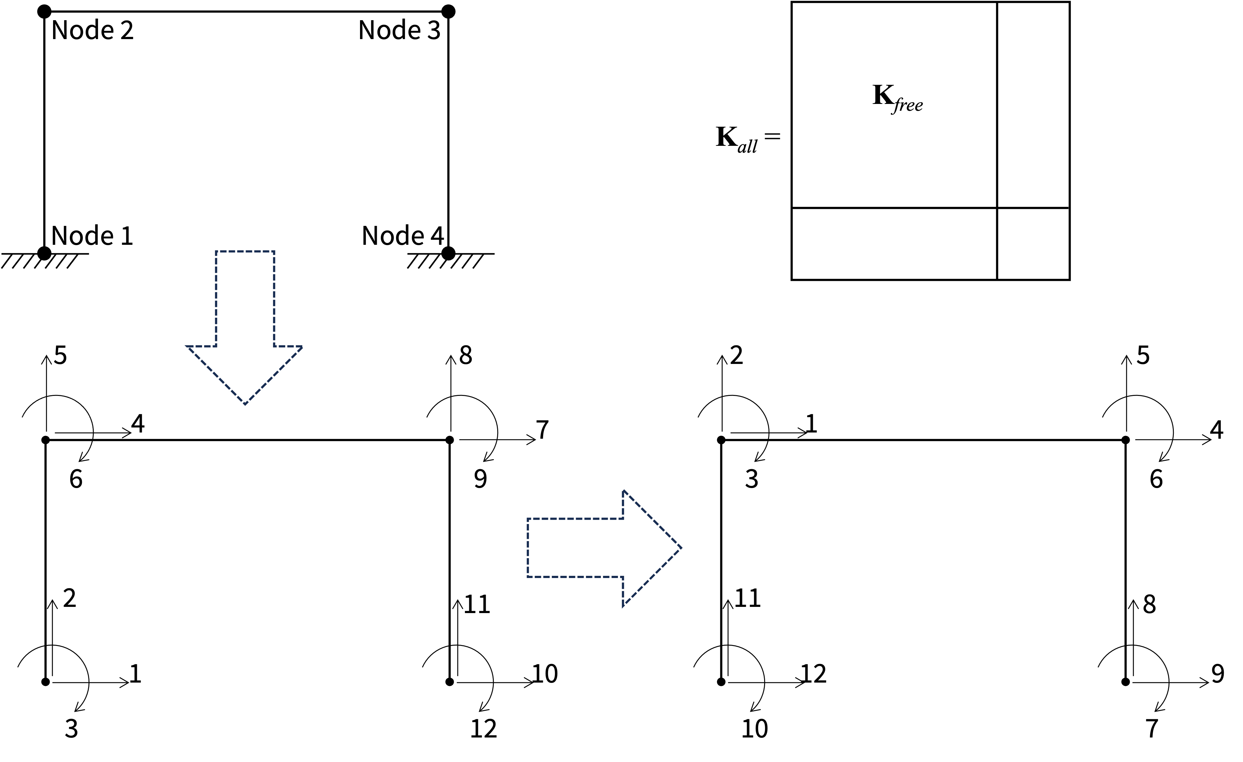
The top-left frame in that figure shows the node numbering implied by the input in Listing 2.1. The resulting unaltered DOF numbering appears in the lower-left. In the lower-right frame in Figure 2.1, the first fixed DOF is given the last DOF number, the first free DOF is given the first DOF number, and so forth. That is the DOF numbering resulting from this algorithm:
class model(model):
    def dofNumberer(self):
        nnodes = np.size(self.CONSTRAINTS, 0)
        ndof = np.size(self.CONSTRAINTS, 1)
        n = nnodes * ndof
        DOF = np.zeros((np.size(self.CONSTRAINTS, 0), np.size(self.CONSTRAINTS, 1)), dtype = int)
        k = 0
        for i in range(nnodes):
            for j in range(ndof):
                if self.CONSTRAINTS[i,j] == 0:
                    DOF[i,j] = k
                    k = k + 1
                else:
                    n = n - 1
                    DOF[i,j] = n
        nfree = k
        nfixed = n
        return DOF, nfree, nfixed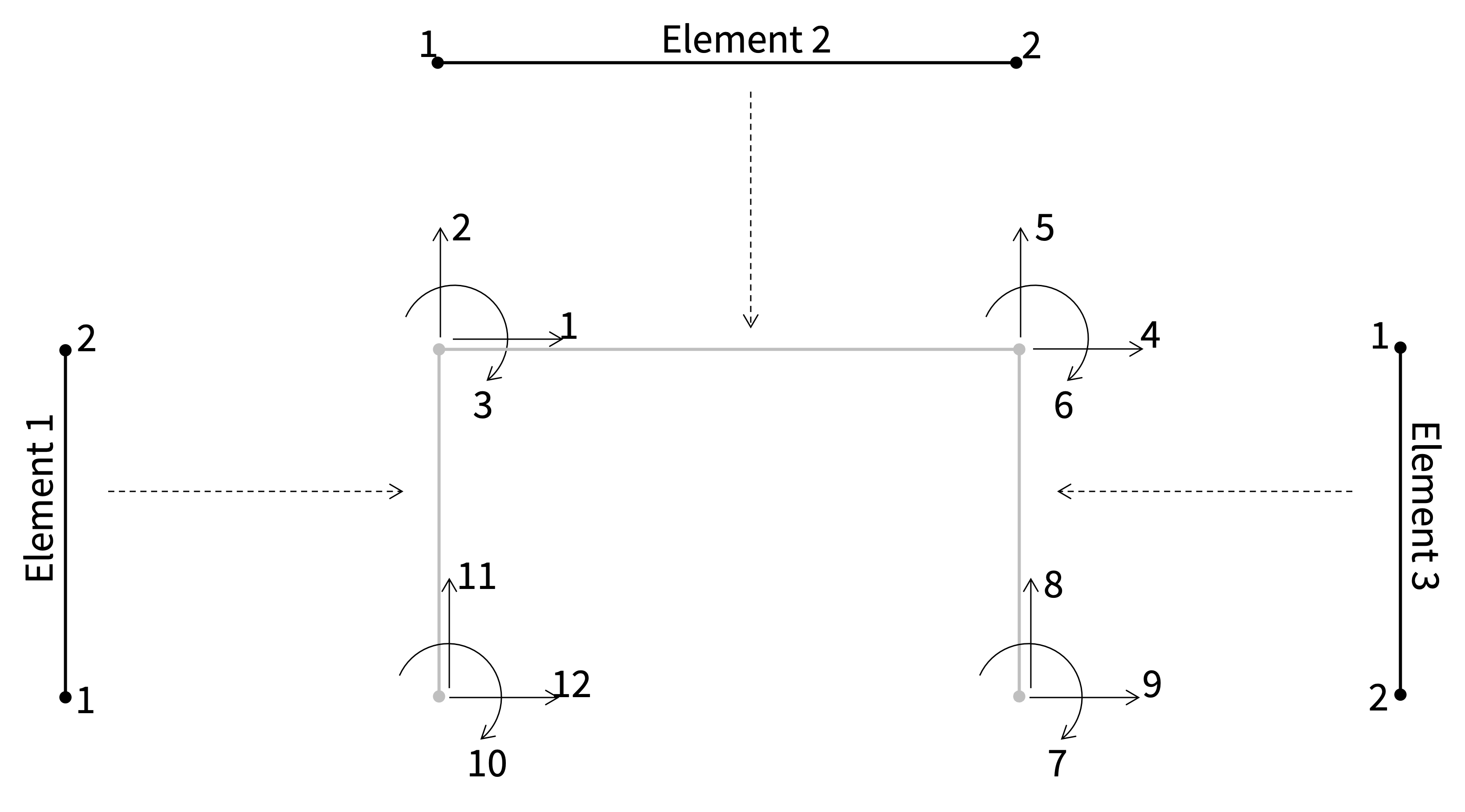
Next, each element is connected to the new node numbering provided in the DOF array from the previous algorithm. Figure 2.2 highlights the element connectivity implied by input given in Listing 2.1. For instance, that input says that the first node of Element 3 is the top-right node of the frame, i.e., the third node of the frame. That kind of information is employed in the following generic algorithm:
class model(model):
    def idNumberer(self):
        nelem = len(self.ELEMENTS)
        numNodesPerElement = 2
        dofnod = np.size(self.DOF, 1)
        ID = np.zeros((nelem, 1+numNodesPerElement*dofnod), dtype = int)
        for i in range(nelem):
            num = 0
            lid = []
            for j in range(numNodesPerElement):
                entry = len(self.ELEMENTS[i][:]) - 2 + j
                nod = int(self.ELEMENTS[i][entry])
                if nod > 0:
                    lid.extend(self.DOF[nod-1,:])
                    num = num + dofnod
            ID[i, 0] = num
            ID[i, 1:len(lid)+1] = lid
        return ID
The result, verified by running Listing 2.7 near the end of this chapter is an ID array with the composition \[
\begin{aligned}
ID &=
\begin{Bmatrix}
\mathrm{Element}\; 1 \\
\mathrm{Element}\; 2 \\
\mathrm{Element}\; 3
\end{Bmatrix} \\[10pt]
&=
\begin{Bmatrix}
\{\mathrm{Node \; 1 \; DOFs} \}, \{\mathrm{Node \; 2 \; DOFs} \} \\
\{\mathrm{Node \; 2 \; DOFs} \}, \{\mathrm{Node \; 3 \; DOFs} \} \\
\{\mathrm{Node \; 3 \; DOFs} \}, \{\mathrm{Node \; 4 \; DOFs} \}
\end{Bmatrix} \\[10pt]
&=
\begin{Bmatrix}
\{12, 11, 10\}, \{1, 2, 3\} \\
\{1, 2, 3\}, \{4, 5, 6\} \\
\{4, 5, 6\}, \{9, 8, 7\}
\end{Bmatrix}
\end{aligned}
\tag{2.1}\]
where the DOF numbers match those in Figure 2.2. When this is later compared with the result of running the algorithm, two discrepancies are observed:
- Python starts counting at
0; therefore, all DOF numbers will be one less than in Equation 2.1 - The algorithm in Listing 2.7 prepends, in every row, the total number of DOFs that the element is connected to, in this case six, three at each node
Next, a member function involved in the communication between the structural analysis algorithm and the elements is addressed. The algorithm labelled localize below is called by the structural analysis, for each element individually, to accomplish three things:
- Get the row of the
IDarray created in Figure 2.2 for the present element (id) - Get the coordinates of the element ends (
xyz) - Get the displacements and rotations along the element DOFs from the \(\mathbf{u}_{\mathrm{all}}\) vector of the structure, with both fixed and free DOFs, i.e., get
uglobalfromuall
class model(model):
    def localize(self, elem, uall):
        n = self.ID[elem, 0]
        id = self.ID[elem, 1:n+1]
        con = self.ELEMENTS[elem][:]
        xyz = []
        numNodesPerElement = 2
        for i in range(numNodesPerElement):
            nod = int(con[len(con)-2+i])
            if nod > 0:
                xyz.append(self.NODES[nod-1,:])
        xyz = np.array(xyz)
        if len(uall) == 0:
            uglobal = 0
        else:
            uglobal = uall[id]
        return id, xyz, uglobal
The last member function of the structural model, as it is introduced now, is simpler than the previous ones. The getData function shown below simply provides the number of DOFs, together with the mass matrix and the load vector that stems from nodal loads. It is observed below that the DOF array established earlier is employed to assemble both. This is done once and for all by the structural model object, contrasting with the stiffness matrix and internal force vector. This acknowledges that, in nonlinear analysis, the stiffness matrix and internal force vector change during the analysis, needing to be repeatedly assembled. Details are provided in subsequent chapters.
class model(model):
    def getData(self):
        nnodes = np.size(self.DOF,0)
        numdofnod = np.size(self.DOF,1)
        ntot = nnodes * numdofnod

        F = np.zeros(ntot)
        if np.size(self.NODELOAD, 1) > 0:
            for i in range(nnodes):
                id = self.DOF[i,:]
                F[id] = F[id] + self.NODELOAD[i,:]

        M = np.zeros(ntot)
        if np.size(self.NODEMASS, 1) > 0:
            for i in range(nnodes):
                id = self.DOF[i,:]
                M[id] = M[id] + self.NODEMASS[i,:]
        M = np.diag(M)

        return self.nfree, ntot, F, M, self.ELEMLIST
Several types of elements, cross-sections, and material models are introduced later in this book, enhanced with response sensitivity calculations. For now, only the constructor of the linear frame element, i.e., Element 5, is provided. This is necessary to test the structural model class in this chapter:
class element5():
    def __init__(self, E, A, I, q, elno):
        self.no = elno
        self.E  = E
        self.A  = A
        self.I  = I
        self.q  = q
2.4 Testing the Model
The following member function creates a rudimentary plot of the structure. Node numbers are red and element numbers are blue. The exception is green numbers for some diagonal elements; this is a simple attempt at avoiding overlapping element numbers when plotting cross-braced truss structures later in this book:
class model(model):
    def plotModel(self):
        plt.figure()
        o = np.max(np.abs(self.NODES))*1e-2 # Offset numbers in plot
        nelem = len(self.ELEMENTS)
        for i in range(nelem):
            node1 = int(self.ELEMENTS[i][len(self.ELEMENTS[i][:])-2])
            node2 = int(self.ELEMENTS[i][len(self.ELEMENTS[i][:])-1])
            x1 = self.NODES[node1-1, 0]; x2 = self.NODES[node2-1, 0]
            y1 = self.NODES[node1-1, 1]; y2 = self.NODES[node2-1, 1]
            plt.plot([x1, x2], [y1, y2], 'ko-')
            midx=(x1+x2)/2; midy=(y1+y2)/2
            if x2-x1==y1-y2:
                plt.text(midx+o, midy-3*o, str(i+1), fontsize=12, color='g')
            else:
                plt.text(midx+o, midy+o, str(i+1), fontsize=12, color='b')
        nnodes = len(self.NODES)
        for i in range(nnodes):
            plt.text(self.NODES[i,0]+o, self.NODES[i,1]+o, str(i+1), fontsize=12, color='r')
        plt.axis('equal')
        plt.show()
That plotting function is executed here, for the portal frame input provided in Listing 2.1, after first creating the structural model:
structuralModel = model(input)
structuralModel.plotModel()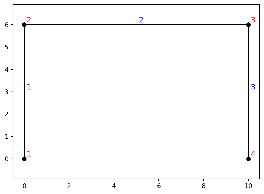
The member functions dofNumberer(), idNumberer(), and localize(), presented in Listing 2.6, Listing 2.7, and Listing 2.8, are key to the efficient assembly of the stiffness matrix, as well as the iterations in nonlinear analysis. The first of those functions confirm the node numbering in Figure 2.1:
DOF, nfree, nfixed = structuralModel.dofNumberer()
print(f"The model has {nfree+nfixed} DOFs: {nfree} are free and {nfixed} are fixed")
print("The DOF array with renumbered DOFs is:\n", DOF)
The model has 12 DOFs: 6 are free and 6 are fixed
The DOF array with renumbered DOFs is:
[[11 10 9]
[ 0 1 2]
[ 3 4 5]
[ 8 7 6]]Next, the output from the idNumberer function confirms Equation 2.1, with the previously mentioned caveats about Python counting from 0 and the first column of the ID array containing the number of DOFs in the element:
ID = structuralModel.idNumberer()
print("The ID array is:\n", ID)
The ID array is:
[[ 6 11 10 9 0 1 2]
[ 6 0 1 2 3 4 5]
[ 6 3 4 5 8 7 6]]