from Chapter12code import *13 Synthetic Ground Motions
This chapter maintains the goal of calculating response sensitivities. However, now it is derivatives with respect to variables given to generators of artificial ground motions that are of interest. Master’s student Saadatmand (2024) was instrumental in deriving and implementing these derivatives under my supervision. Two types of synthetic ground motions are considered in the sections below. The first employing the frequency domain of stochastic process analysis, the other the time domain.
13.1 Spectral Approach
The energy released in an earthquake results in acceleration of the ground in the vicinity of the rupture. The ground acceleration can be regarded as a stochastic process, with energy quantified by a power spectral density, or spectrum for short. A one-sided spectrum, i.e., for positive frequency values, is denoted by \(S(\omega)\), where \(\omega=\) frequency in radians per second. Energy is quantified by the spectrum as variance, i.e., the second central statistical moment introduced in Chapter 1. The area underneath \(S(\omega)\) is the variance of the zero mean random variable that we can imagine existing at any given time instant. If we assume that the random variable has the Normal distribution, and that \(S(\omega)\) is constant along the time axis, then we have the popular stationary Gaussian stochastic process. Such a model is less appropriate for earthquake ground motion than, say, ocean wave loading on offshore installations. However, a modulation technique presented below introduces the non-stationarity that is a characteristic of ground motions.
There exists a rich theory of stochastic processes, and various spectra are formulated for different applications. In earthquake engineering, various versions of the Kanai-Tajimi spectrum are used because it represents the acceleration response of a single-DOF system. One can think of this spectrum as the response of the soil to a white noise rupture at the bedrock level. White noise means uniform excitation at all frequencies. The expression for the Kanai-Tajimi spectrum employed in this chapter is \[ S(\omega) = S_0 \cdot \frac{\omega_g^4 + (2 \zeta_g \omega_g \omega)^2}{\left(\omega_g^2 - \omega^2 \right)^2 + (2 \zeta_g \omega_g \omega)^2} \tag{13.1}\]
where \(S_0=\) intensity of the bedrock white noise, \(\omega_g=\) dominant soil frequency, and \(\zeta_g=\) soil damping. A reasonable damping choice is \(\zeta_g = \frac{\omega_g}{25}\) with \(\omega_g=5\)rad/sec for soft soil, \(\omega_g=10\)rad/sec for medium soil, and \(\omega_g=15\)rad/sec or higher for firm soil. Values as high as \(\omega_g=25\)rad/sec is seen in the literature, but then another choice of damping value must be made. Various models exist for the ground motion intensity, \(S_0\). They all contain the variable \(\sigma_g^2\), to highlight that the ground motion intensity is measured by statistical variance. The expression employed here is
\[ S_0 = \frac{4 \sigma_g^2 \zeta_g}{\omega_g (4 \zeta_g^2 +1)} \tag{13.2}\]
That expression gives a standard deviation of the ground acceleration that is independent of the value of \(\omega_g\) and not highly dependent on \(\zeta_g\). For high damping values, the standard deviation of the ground motion is around \(1.7 \cdot \sigma_g\); for low damping values it is around \(1.77 \cdot \sigma_g\). The intensity and soil conditions specified here, as a demonstration, are
sigma_g = 2/1.75     # m/s^2
omega_g = 15         # rad/sec
zeta_g = omega_g/25  # Dimensionless
In the following, the frequency axis is discretized and the variance in each interval is utilized. To that end, the discretization choice is
minFreq = 0
maxFreq = 5*omega_g
nblocks = 200
omega = np.linspace(minFreq, maxFreq, nblocks)
That gives the following plot of the Kanai-Tajimi spectrum, implementing the expressions in Equation 13.1 and Equation 13.2:
S0 = 4 * sigma_g**2 * zeta_g / (omega_g * (4 * zeta_g**2 + 1))
S = S0 * (omega_g**4 + (2 * zeta_g * omega_g * omega)**2) / ((omega_g**2 - omega**2)**2 + (2 * zeta_g * omega_g * omega)**2)
plt.figure()
plt.plot(omega, S, 'k-', linewidth=1.0)
plt.xlabel("$\\omega$ [rad/sec.]")
plt.ylabel("Kanai-Tajimi spectrum, $S(\\omega)$")
plt.grid(True)
plt.show()
from scipy.integrate import simpson
print(f"Standard deviation of ground acceleration: {np.sqrt(simpson(S, x=omega)):.2f}m/s^2")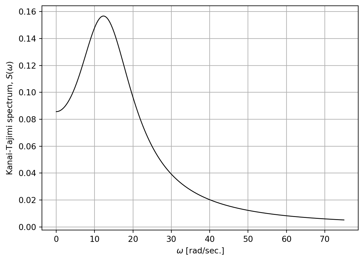
Standard deviation of ground acceleration: 1.93m/s^2Notice that the square root of the area underneath the spectrum is printed below the plot. The variance in each interval of the discretized spectrum is
\[ \sigma_i^2 = \Delta\omega \cdot S(\omega_i) \tag{13.3}\]
where \(i\) counts the \(N\) intervals that the spectrum is divided into. In turn, that gives the standard deviation of the Normal random variables, \(A_i\), in the following sum that generates the ground acceleration, with one sine wave from each interval of the discretized spectrum:
\[ \ddot{u}_g(t) = \sqrt{2} \cdot \sum_{i=1}^{N} A_i \cdot \mathrm{sin}(\omega_i t + \phi_i) \tag{13.4}\]
The factor \(\sqrt{2}\) is introduced because the standard deviation of a sine wave is \(\frac{1}{\sqrt{2}}\). In Equation 13.4, \(\phi_i\) is a random phase angle, different for each sine wave, generated randomly between \(0\) and \(2\pi\). The ground acceleration generated in that way has two issues not matching actual ground motions. First, it is stationary; this is addressed below by means of a modulating function. Second, it is likely to have residual velocity and displacement at the end of the ground shaking. It is possible to add a slowly varying function to Equation 13.4 to remedy this. However, that added function would make the sensitivity analysis slightly more convoluted and is therefore neglected in this version of the book.
In subsequent sensitivity derivations, we need \(\frac{\partial A_i}{\partial x}\), where \(x\) represents \(\sigma_g\), \(\omega_g\), or \(\zeta_g\). For that reason, it is helpful to generate realizations of \(A_i\) in the following manner:
- Generate the outcome of a Standard Normal variable, \(y_i\), which does not depend on \(\sigma_g\)
- Employ the probability transformation in Equation 6.2 to obtain \(A_i = F^{-1}(\Phi(y_i))\), where \(F^{-1}(\,)\) is the Normal inverse CDF with zero mean and standard deviation \(\sigma_i\) from Equation 13.3. Importantly, the derivative of \(F^{-1}(\,)\) with respect to \(\sigma_g\) is available, as shown later.
That sequence of random number generation is employed here:
from scipy.stats import norm
duration = 25.0
dt = 0.01
numTimePoints = int(duration / dt) + 1
t = np.linspace(0, dt * (numTimePoints-1), numTimePoints)
phi = 2*np.pi*np.random.uniform(low=0.0, high=1.0, size=nblocks)
groundAcceleration = np.zeros(len(t))
y = np.random.normal(loc=0.0, scale=1.0, size=nblocks)
deltaOmega = (maxFreq-minFreq)/nblocks
intervalStdv = np.sqrt(deltaOmega * S)
for i in range(nblocks):
    standardNormalCDFofy = norm.cdf(y[i], 0, 1)
    A = norm.ppf(standardNormalCDFofy, 0, intervalStdv[i])
    groundAcceleration += np.sqrt(2) * A * np.sin(omega[i] * t + phi[i])
The generated ground acceleration is plotted here:
plt.figure()
plt.plot(t, groundAcceleration, 'k-', linewidth=1.0)
plt.xlabel("Time [sec.]")
plt.ylabel("$\\ddot{u}_g(t)$ [$\\frac{m}{s^2}$]")
plt.grid(True)
plt.show()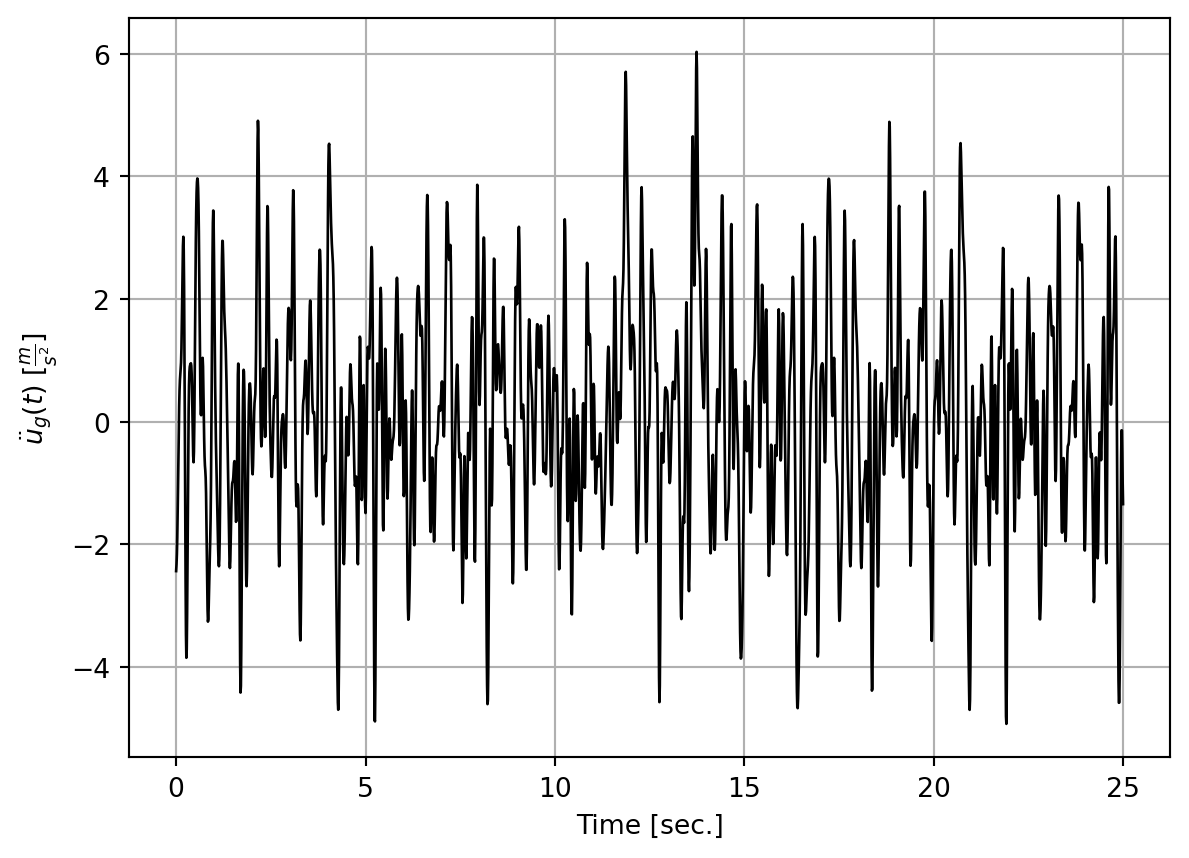
13.1.1 Modulation
A trapezoidal modulating function is utilized here to make the ground motion non-stationary. It is defined by the function
def trapezoidalModulatingFunction(t, t1, t2, t3, t4):
    if t < t1:
        return 0.0
    elif t < t2:
        return (t - t1) / (t2 - t1)
    elif t < t3:
        return 1.0
    elif t < t4:
        return 1.0 - (t - t3) / (t4 - t3)
    else:
        return 0.0
Here is a plot of that modulating function, for selected input values:
t1 = 0
t2 = 3
t3 = 10
t4 = duration
modFunc = []
t = np.linspace(0, duration, numTimePoints)
for i in range(numTimePoints):
    modFunc.append(trapezoidalModulatingFunction(t[i], t1, t2, t3, t4))
plt.figure()
plt.plot(t, modFunc, 'k-', linewidth=1.0)
plt.xlabel("Time [sec]")
plt.ylabel("Modulating function")
plt.show()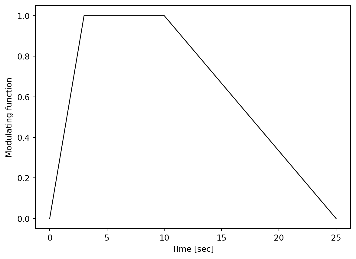
When that modulating function is multiplied with the ground motion created earlier, the result looks like this:
modulatedGroundAcceleration = groundAcceleration * modFunc
plt.figure()
plt.plot(t, modulatedGroundAcceleration, 'k-', linewidth=1.0)
plt.xlabel("Time [sec.]")
plt.ylabel("$\\ddot{u}_g(t)$ [$\\frac{m}{s^2}$]")
plt.grid(True)
plt.show()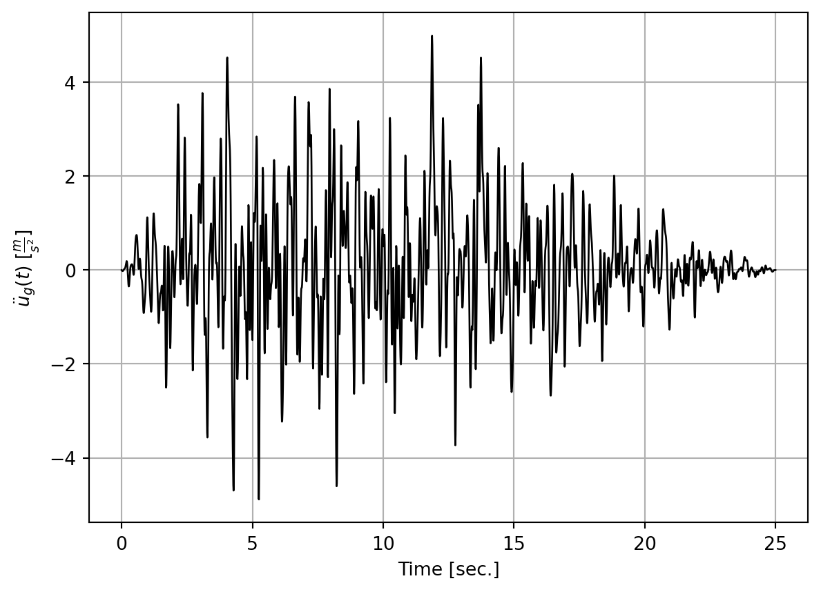
13.1.2 Differentiation
Equation 13.4 is now differentiated in order to obtain first-order response derivatives with respect to \(\sigma_g\), \(\omega_g\), and \(\zeta_g\). Those variables only affect \(A_i\); they do not affect \(\omega_i\) and \(\phi_i\). For that reason, the sought derivative is first expressed by the chain rule of differentiation:
\[ \frac{\partial \ddot{u}_g(t)}{\partial x} = \frac{\partial \ddot{u}_g(t)}{\partial A_i}\frac{\partial A_i}{\partial \sigma_i} \frac{\partial \sigma_i}{\partial x} \tag{13.5}\]
where \(\sigma_i\) is defined in Equation 13.3. The first derivative in the right-hand side of Equation 13.5 is, from Equation 13.4,
\[ \frac{\partial \ddot{u}_g(t)}{\partial A_i} = \sqrt{2} \cdot \mathrm{sin}(\omega_i t + \phi_i) \tag{13.6}\]
To obtain the second derivative in the right-hand side of Equation 13.5 we take advantage of the two-step ground motion generation scheme described earlier with the formula \(A_i = F^{-1}(\Phi(y_i))\). The derivative of the inverse Normal CDF with zero mean and standard deviation \(\sigma_i\) with respect to \(\sigma_i\) gives
\[ \frac{\partial A_i}{\partial \sigma_i} = -\sqrt{2} \cdot \mathrm{invErr}(1-2\Phi(y_i)) \tag{13.7}\]
where \(\mathrm{invErr}(\,)=\) inverse of the error function known from statistics. The third derivative in the right-hand side of Equation 13.5 requires the differentiation of Equation 13.3, which again requires the differentiation of the Kanai-Tajimi spectrum:
\[ \frac{\partial \sigma_i}{\partial x} = \sqrt{\Delta\omega} \cdot \frac{1}{2 \sqrt{S(\omega_i)}} \cdot \frac{\partial S(\omega_i)}{\partial x} \tag{13.8}\]
Those derivatives appear below, in a function that generates the ground motion, now including first-order sensitivity calculations:
def spectralGroundMotion(duration, dt, minFreq, maxFreq, nblocks, sigma_g, omega_g, zeta_g, modFunc, t1, t2, t3, t4, seed):
    from scipy.special import erfinv
    from scipy.stats import norm
    deltaOmega = (maxFreq-minFreq)/nblocks
    omega = np.linspace(minFreq+0.5*deltaOmega, maxFreq-0.5*deltaOmega, nblocks)
    S0 = 4 * sigma_g**2 * zeta_g / (omega_g * (4 * zeta_g**2 + 1))
    S = S0 * (omega_g**4 + (2 * zeta_g * omega_g * omega)**2) / ((omega_g**2 - omega**2)**2 + (2 * zeta_g * omega_g * omega)**2)

    dSdsigma = (8*sigma_g*zeta_g*(omega_g**4 + 4*omega_g**2*omega**2*zeta_g**2))/(omega_g*(1 + \
                4*zeta_g**2)*((omega_g**2 - omega**2)**2 + 4*omega_g**2*omega**2*zeta_g**2))

    dSdomega = (-4*sigma_g**2*zeta_g*(4*omega_g*(omega_g**2 - omega**2) + \
                8*omega_g*omega**2*zeta_g**2)*(omega_g**4 + 4*omega_g**2*omega**2*zeta_g**2))/(omega_g*(1 \
                + 4*zeta_g**2)*((omega_g**2 - omega**2)**2 + 4*omega_g**2*omega**2*zeta_g**2)**2) + \
                (4*sigma_g**2*zeta_g*(4*omega_g**3 + 8*omega_g*omega**2*zeta_g**2))/(omega_g*(1 + \
                4*zeta_g**2)*((omega_g**2 - omega**2)**2 + 4*omega_g**2*omega**2*zeta_g**2)) - \
                (4*sigma_g**2*zeta_g*(omega_g**4 + 4*omega_g**2*omega**2*zeta_g**2))/(omega_g**2*(1 \
                + 4*zeta_g**2)*((omega_g**2 - omega**2)**2 + 4*omega_g**2*omega**2*zeta_g**2))

    dSdzeta = (-32*omega_g*sigma_g**2*omega**2*zeta_g**2*(omega_g**4 + \
                4*omega_g**2*omega**2*zeta_g**2))/((1 + 4*zeta_g**2)*((omega_g**2 - omega**2)**2 + \
                4*omega_g**2*omega**2*zeta_g**2)**2) + (32*omega_g*sigma_g**2*omega**2*zeta_g**2)/((1 + \
                4*zeta_g**2)*((omega_g**2 - omega**2)**2 + 4*omega_g**2*omega**2*zeta_g**2)) - \
                (32*sigma_g**2*zeta_g**2*(omega_g**4 + 4*omega_g**2*omega**2*zeta_g**2))/(omega_g*(1 \
                + 4*zeta_g**2)**2*((omega_g**2 - omega**2)**2 + 4*omega_g**2*omega**2*zeta_g**2)) + \
                (4*sigma_g**2*(omega_g**4 + 4*omega_g**2*omega**2*zeta_g**2))/(omega_g*(1 + \
                4*zeta_g**2)*((omega_g**2 - omega**2)**2 + 4*omega_g**2*omega**2*zeta_g**2))

    intervalStdv = np.sqrt(deltaOmega * S)
    np.random.seed(seed)
    phi = 2 * np.pi * np.random.uniform(low=0.0, high=1.0, size=nblocks)
    numTimePoints = int(duration / dt) + 1
    t = np.linspace(0, dt * (numTimePoints-1), numTimePoints)
    groundAcceleration = np.zeros(len(t))
    daccdsigma = np.zeros(len(t))
    daccdomega = np.zeros(len(t))
    daccdzeta = np.zeros(len(t))
    np.random.seed(seed+1)
    y = np.random.normal(loc=0.0, scale=1.0, size=nblocks)
    for i in range(nblocks):
        standardNormalCDFofy = norm.cdf(y[i], 0, 1)
        A = norm.ppf(standardNormalCDFofy, 0, intervalStdv[i])
        groundAcceleration += np.sqrt(2) * A * np.sin(omega[i] * t + phi[i])
        daccdA = np.sqrt(2) * np.sin(omega[i] * t + phi[i])
        dAdsigma = -np.sqrt(2) * erfinv(1 - 2 * standardNormalCDFofy)
        dsigmadsigma = np.sqrt(deltaOmega) / (2 * np.sqrt(S[i])) * dSdsigma[i]
        dsigmadomega = np.sqrt(deltaOmega) / (2 * np.sqrt(S[i])) * dSdomega[i]
        dsigmadzeta = np.sqrt(deltaOmega) / (2 * np.sqrt(S[i])) * dSdzeta[i]
        daccdomega += daccdA * dAdsigma * dsigmadomega
        daccdsigma += daccdA * dAdsigma * dsigmadsigma
        daccdzeta += daccdA * dAdsigma * dsigmadzeta
    for i in range(numTimePoints):
        modulation = modFunc(t[i], t1, t2, t3, t4)
        groundAcceleration[i] = groundAcceleration[i] * modulation
        daccdsigma[i] = daccdsigma[i] * modulation
        daccdomega[i] = daccdomega[i] * modulation
        daccdzeta[i] = daccdzeta[i] * modulation
    metersPerSec2GroundMotionMatrix = np.concatenate(([t], [groundAcceleration], [daccdsigma], [daccdomega], [daccdzeta]), axis=0)
    return metersPerSec2GroundMotionMatrix
Here is a plot of the generated ground motion:
seed = 1
gmMatrix = spectralGroundMotion(duration, dt, minFreq, maxFreq, nblocks, sigma_g, omega_g, zeta_g, trapezoidalModulatingFunction, t1, t2, t3, t4, seed)
plt.figure()
plt.plot(gmMatrix[0], gmMatrix[1], 'k-', linewidth=1.0)
plt.xlabel("Time [sec.]")
plt.ylabel("$\\ddot{u}_g(t)$ [$\\frac{m}{s^2}$]")
plt.grid(True)
plt.show()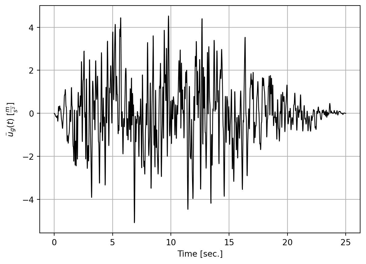
Here are the sensitivities with respect to the three input variables:
timeWindow = range(int(0.2*len(gmMatrix[0])), int(0.3*len(gmMatrix[0])))
plt.figure()
plt.plot(gmMatrix[0, timeWindow], gmMatrix[2, timeWindow]*0.1*sigma_g, 'b-', linewidth=1.0, label='$\\frac{\\partial \\ddot{u}_g}{\\partial \\sigma_g}$')
plt.plot(gmMatrix[0, timeWindow], gmMatrix[3, timeWindow]*0.1*omega_g, 'r-', linewidth=1.0, label='$\\frac{\\partial \\ddot{u}_g}{\\partial \\omega_g}$')
plt.plot(gmMatrix[0, timeWindow], gmMatrix[4, timeWindow]*0.1*zeta_g, 'g-', linewidth=1.0, label='$\\frac{\\partial \\ddot{u}_g}{\\partial \\zeta_g}$')
plt.xlabel("Time [sec.]")
plt.grid(True)
plt.legend(loc='upper right')
plt.show()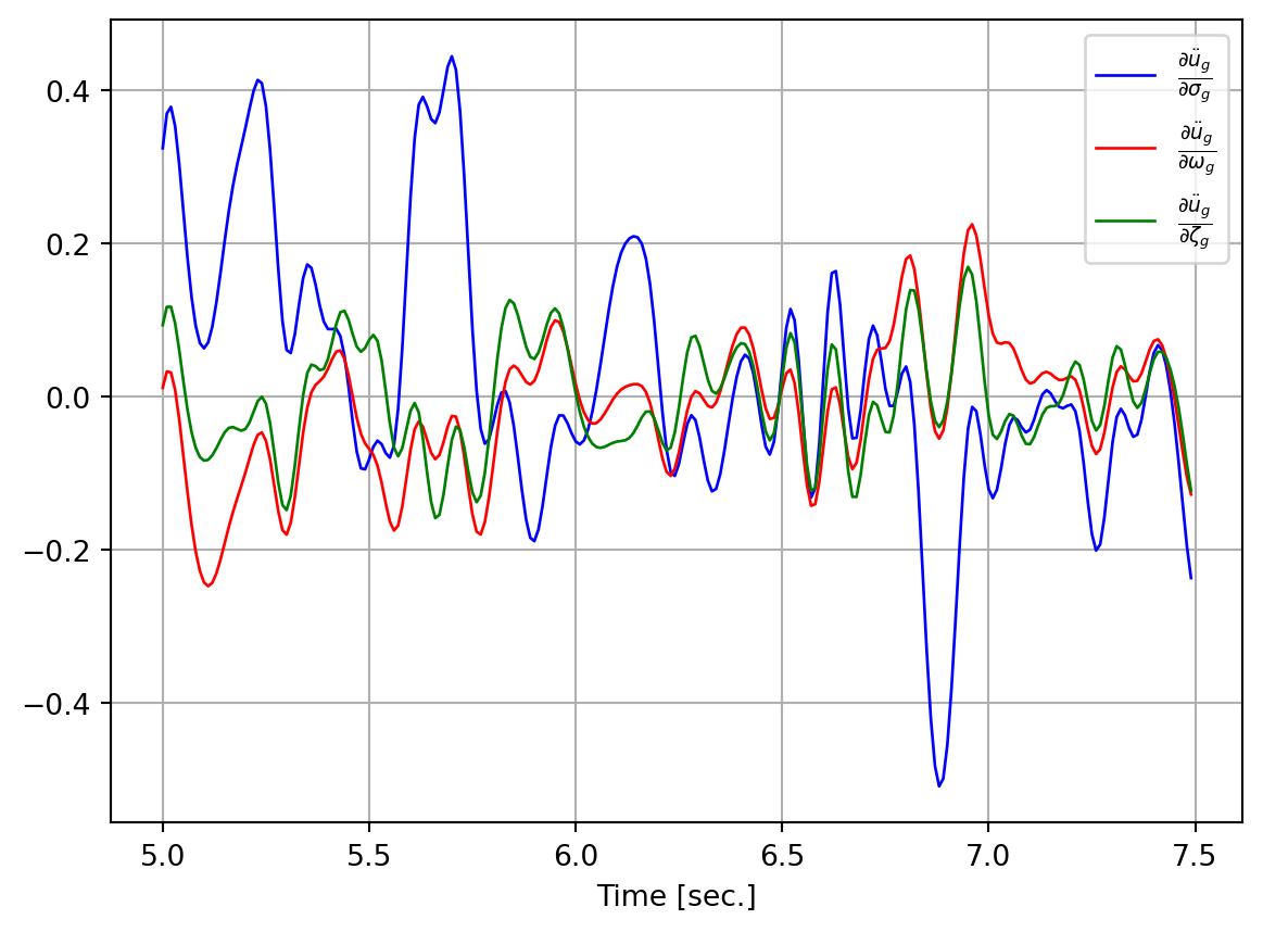
13.2 Filtered White Noise
This ground motion model more explicitly mimics the energy pulses emanating from the rupture at bedrock, filtered through the soil, resulting in ground acceleration. It is expressed as
\[ \ddot{u}_g(t) = s \cdot \sigma_g \cdot \sum_{i=1}^{N} y_i \cdot h(t - t_i) \tag{13.9}\]
where \(s=\) scaling factor, \(N=\) number of pulses spread along the time axis, \(y_i=\) Standard Normal random variable, \(h(\,)=\) filter, and \(t_i=\) time of pulse number \(i\). The value of \(s\) should be calculated so that \(\sigma_g\) is the standard deviation of the stochastic process. This is possible, for example by numerical integration, and \(s\) then is a function of input parameters, including the temporal distance between the pulses. A simpler approach is selected in this chapter, simply having \(s\) as a user-given constant, independent of other input to the model.
Statistical reasons dictate that the process must be differentiable, which means that each filter must start at zero intensity at \(t_i\). That is one reason why the displacement impulse response function known from single-DOF dynamics is viable as filter. Keeping only the exponential and sine functions, the expression is
\[ h(t) = e^{-\omega_g \cdot \zeta_g \cdot t} \cdot \mathrm{sin}\left(\omega_g \cdot \sqrt{1-\zeta_g^2} \cdot t \right) \tag{13.10}\]
The derivative of this ground motion model with respect to the intensity parameter is
\[ \frac{\partial \ddot{u}_g(t)}{\partial \sigma_g} = s \cdot \sum_{i=1}^{N} y_i \cdot h(t - t_i) \tag{13.11}\]
The derivative with respect to soil frequency and damping is
\[ \frac{\partial \ddot{u}_g(t)}{\partial x} = s \cdot \sigma_g \cdot \sum_{i=1}^{N} y_i \cdot \frac{\partial h(t - t_i)}{\partial x} \tag{13.12}\]
where the derivative of the filter is implemented in the following
def h(omega_g, zeta_g, t):
    if t > 0:
        return np.exp(-omega_g * zeta_g * t) * np.sin(omega_g * np.sqrt(1-zeta_g**2) * t)
    else: return 0

def dhdOmega(omega_g, zeta_g, t):
    if t > 0:
        return -t*zeta_g*np.exp(-omega_g*t*zeta_g)*np.sin(omega_g*t*np.sqrt(1 - zeta_g**2)) + t*np.sqrt(1 - zeta_g**2)*np.exp(-omega_g*t*zeta_g)*np.cos(omega_g*t*np.sqrt(1 - zeta_g**2))
    else: return 0

def dhdZeta(omega_g, zeta_g, t):
    if t > 0:
        return -omega_g*t*zeta_g*np.exp(-omega_g*t*zeta_g)*np.cos(omega_g*t*np.sqrt(1 - zeta_g**2))/np.sqrt(1 - zeta_g**2) - omega_g*t*np.exp(-omega_g*t*zeta_g)*np.sin(omega_g*t*np.sqrt(1 - zeta_g**2))
    else: return 0

def filteredWhiteNoise(duration, dt, scaling, sigma_g, omega_g, zeta_g, pulseRate, modFunc, t1, t2, t3, t4, seed):
    pulseSpacing = 1.0 / pulseRate
    numPulses = int(duration * pulseRate)
    sampleRate = int(1.0 / dt)
    numIntervals = int(duration * sampleRate)
    t = np.zeros(numIntervals)
    groundAcceleration = np.zeros(numIntervals)
    daccdsigma = np.zeros(numIntervals)
    daccdomega = np.zeros(numIntervals)
    daccdzeta = np.zeros(numIntervals)
    np.random.seed(seed)
    y = np.random.normal(loc=0.0, scale=1.0, size=numPulses)
    for i in range(numPulses):
        pulseTime = i * pulseSpacing
        for j in range(numIntervals):
            t[j] = j*dt
            modulation = modFunc(t[j], t1, t2, t3, t4)
            groundAcceleration[j] += scaling * sigma_g * y[i] * h(omega_g, zeta_g, t[j]-pulseTime) * modulation
            daccdsigma[j] += scaling * y[i] * h(omega_g, zeta_g, t[j]-pulseTime) * modulation
            daccdomega[j] += scaling * sigma_g * y[i] * dhdOmega(omega_g, zeta_g, t[j]-pulseTime) * modulation
            daccdzeta[j] += scaling * sigma_g * y[i] * dhdZeta(omega_g, zeta_g, t[j]-pulseTime) * modulation
    metersPerSec2GroundMotionMatrix = np.concatenate(([t], [groundAcceleration], [daccdsigma], [daccdomega], [daccdzeta]), axis=0)
    return metersPerSec2GroundMotionMatrix
The generated ground motion is plotted here:
scaling = 4
pulseRate = 10
gmMatrix = filteredWhiteNoise(duration, dt, scaling, sigma_g, omega_g, zeta_g, pulseRate, trapezoidalModulatingFunction, t1, t2, t3, t4, seed)
plt.figure()
plt.plot(gmMatrix[0], gmMatrix[1], 'k-', linewidth=1.0)
plt.xlabel("Time [sec.]")
plt.ylabel("$\\ddot{u}_g(t)$ [$\\frac{m}{s^2}$]")
plt.grid(True)
plt.show()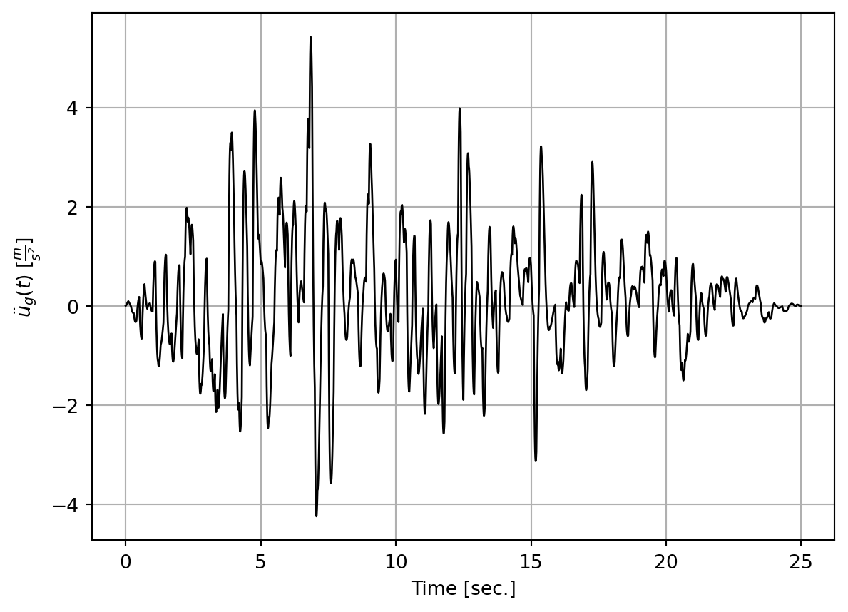
Here are the sensitivities with respect to the three input variables:
plt.figure()
plt.plot(gmMatrix[0, timeWindow], gmMatrix[2, timeWindow]*0.1*sigma_g, 'b-', linewidth=1.0, label='$\\frac{\\partial \\ddot{u}_g}{\\partial \\sigma_g}$')
plt.plot(gmMatrix[0, timeWindow], gmMatrix[3, timeWindow]*0.1*omega_g, 'r-', linewidth=1.0, label='$\\frac{\\partial \\ddot{u}_g}{\\partial \\omega_g}$')
plt.plot(gmMatrix[0, timeWindow], gmMatrix[4, timeWindow]*0.1*zeta_g, 'g-', linewidth=1.0, label='$\\frac{\\partial \\ddot{u}_g}{\\partial \\zeta_g}$')
plt.xlabel("Time [sec.]")
plt.grid(True)
plt.legend(loc='upper left')
plt.show()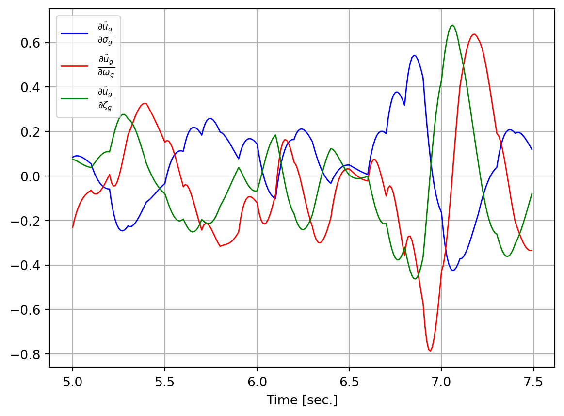
13.3 Structural Response Sensitivity
While it is interesting to view the plots provided above, it is ultimately the structural response that is of primary interest in design. Therefore, a single-DOF dynamic structural model is here created, to demonstrate the use of the functions defined earlier in this chapter:
DDMparameters = [['GroundMotion', 'GivenDerivative', 1],
                 ['GroundMotion', 'GivenDerivative', 2],
                 ['GroundMotion', 'GivenDerivative', 3]]
Tn = 0.5      # seconds
E = 1e4       # N/m
alpha = 0.05  # Dimensionless
uy = 0.03     # m
fy = E * uy   # N
M = (Tn/2/np.pi)**2 * E
dampingRatio = 0.05
Notice that a 0.5 second natural period of vibration is specified. That nonlinear single-DOF system is now subjected to a ground motion generated by the spectral approach. After the analysis is completed, the response sensitivities with respect to \(\sigma_g\), \(\omega_g\) and \(\zeta_g\) are plotted, with a uniform 10% coefficient of variation for the variables:
gmMatrixSpectral = spectralGroundMotion(duration, dt, minFreq, maxFreq, nblocks, sigma_g, omega_g, zeta_g, trapezoidalModulatingFunction, t1, t2, t3, t4, seed)
material = bilinearMaterial(['Bilinear', E, fy, alpha])
t, u, v, a, dudx, dvdx, dadx, dudx2, dnl = nonlinearDynamicSDOFAnalysis(material, M, dampingRatio, gmMatrixSpectral, DDMparameters, 1)
The structural response is plotted below, revealing significant yielding:
plt.figure()
for i in range(1, len(u)):
    if dnl[i] < 1:
        plt.plot([t[i-1], t[i]], [u[i-1], u[i]], 'r-', linewidth=1.0)
    else:
        plt.plot([t[i-1], t[i]], [u[i-1], u[i]], 'k-', linewidth=1.0)
plt.xlabel("Time [sec.]")
plt.ylabel("Displacement [m]")
plt.grid(True)
plt.show()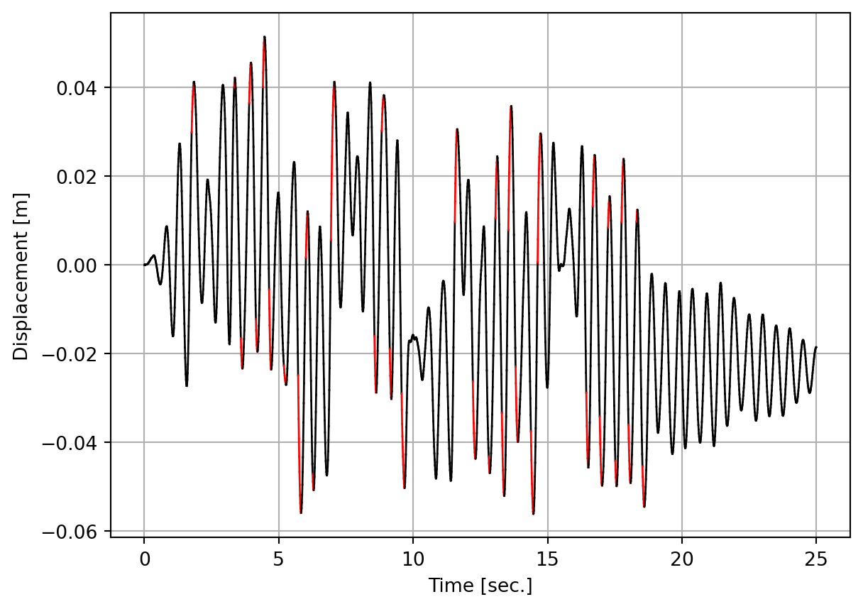
plt.figure()
plt.plot(t, dudx[0]*0.1*sigma_g, 'b-', linewidth=1.0, label='$\\frac{\\partial u}{\\partial \\sigma_g}$')
plt.plot(t, dudx[1]*0.1*omega_g, 'r-', linewidth=1.0, label='$\\frac{\\partial u}{\\partial \\omega_g}$')
plt.plot(t, dudx[2]*0.1*zeta_g, 'g-', linewidth=1.0, label='$\\frac{\\partial u}{\\partial \\zeta_g}$')
plt.xlabel("Time [sec.]")
plt.grid(True)
plt.legend(loc='upper right')
plt.show()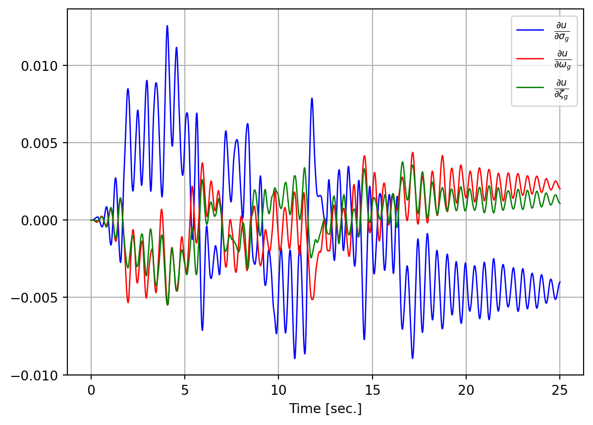
Those response sensitivities are verified in Chapter 14. For comparison, the same analysis is conducted for a ground motion generated by the filtered white noise approach:
gmMatrixWhite = filteredWhiteNoise(duration, dt, scaling, sigma_g, omega_g, zeta_g, pulseRate, trapezoidalModulatingFunction, t1, t2, t3, t4, seed)
material = bilinearMaterial(['Bilinear', E, fy, alpha])
t, u, v, a, dudx, dvdx, dadx, dudx2, dnl = nonlinearDynamicSDOFAnalysis(material, M, dampingRatio, gmMatrixWhite, DDMparameters, 1)
The structural response is plotted below, again revealing significant yielding:
plt.figure()
for i in range(1, len(u)):
    if dnl[i] < 1:
        plt.plot([t[i-1], t[i]], [u[i-1], u[i]], 'r-', linewidth=1.0)
    else:
        plt.plot([t[i-1], t[i]], [u[i-1], u[i]], 'k-', linewidth=1.0)
plt.xlabel("Time [sec.]")
plt.ylabel("Displacement [m]")
plt.grid(True)
plt.show()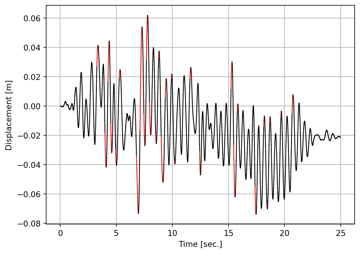
The sensitivities are plotted here for the filtered white noise ground motion:
plt.figure()
plt.plot(t, dudx[0]*0.1*sigma_g, 'b-', linewidth=1.0, label='$\\frac{\\partial u}{\\partial \\sigma_g}$')
plt.plot(t, dudx[1]*0.1*omega_g, 'r-', linewidth=1.0, label='$\\frac{\\partial u}{\\partial \\omega_g}$')
plt.plot(t, dudx[2]*0.1*zeta_g, 'g-', linewidth=1.0, label='$\\frac{\\partial u}{\\partial \\zeta_g}$')
plt.xlabel("Time [sec.]")
plt.grid(True)
plt.legend(loc='upper right')
plt.show()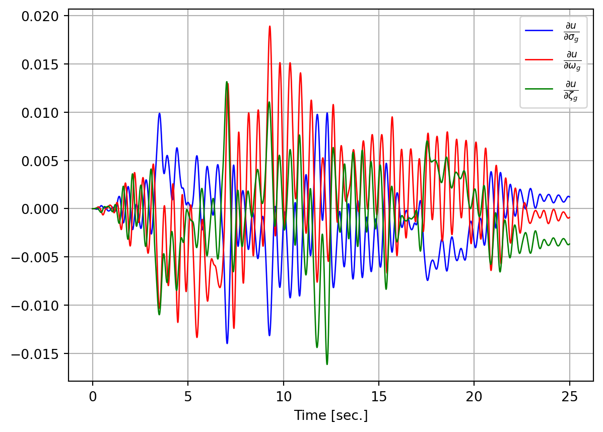
The sensitivity plots above are of course different because different algorithms generated the ground motions. However, it is still interesting to see that the blue line, i.e., \(\frac{\partial u}{\partial \sigma_g}\) seems to be dominant for the spectral approach, while \(\frac{\partial u}{\partial \omega_g}\) appears to stand out a bit more for the filtered white noise approach. This is examined further by increasing the yield strength so that the structure remains linear throughout the analysis:
uy = 1        # m
fy = E * uy   # N
material = bilinearMaterial(['Bilinear', E, fy, alpha])
t, u, v, a, dudx, dvdx, dadx, dudx2, dnl = nonlinearDynamicSDOFAnalysis(material, M, dampingRatio, gmMatrixSpectral, DDMparameters, 1)
The sensitivities for the spectral approach are shown below, now with the code hidden for brevity:
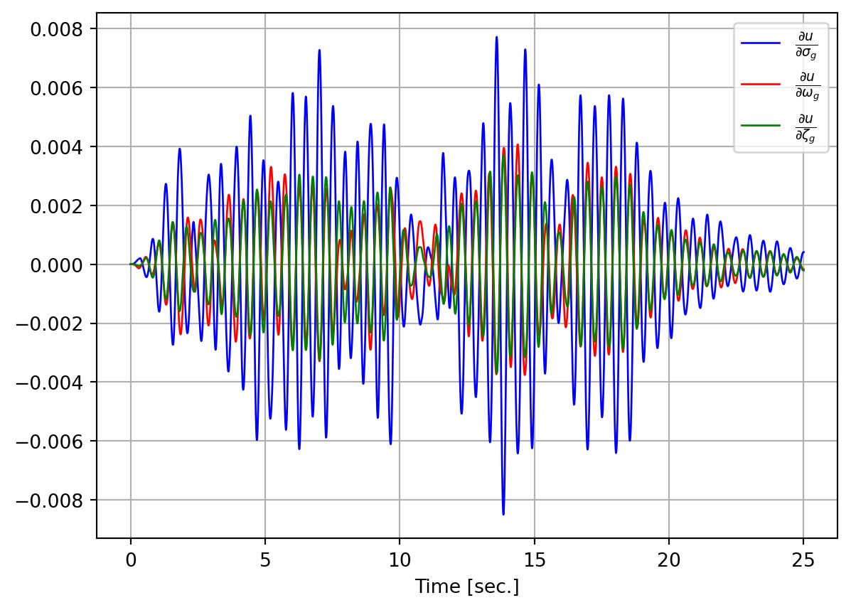
In comparison, the sensitivities for the filtered white noise ground motion now look like this:
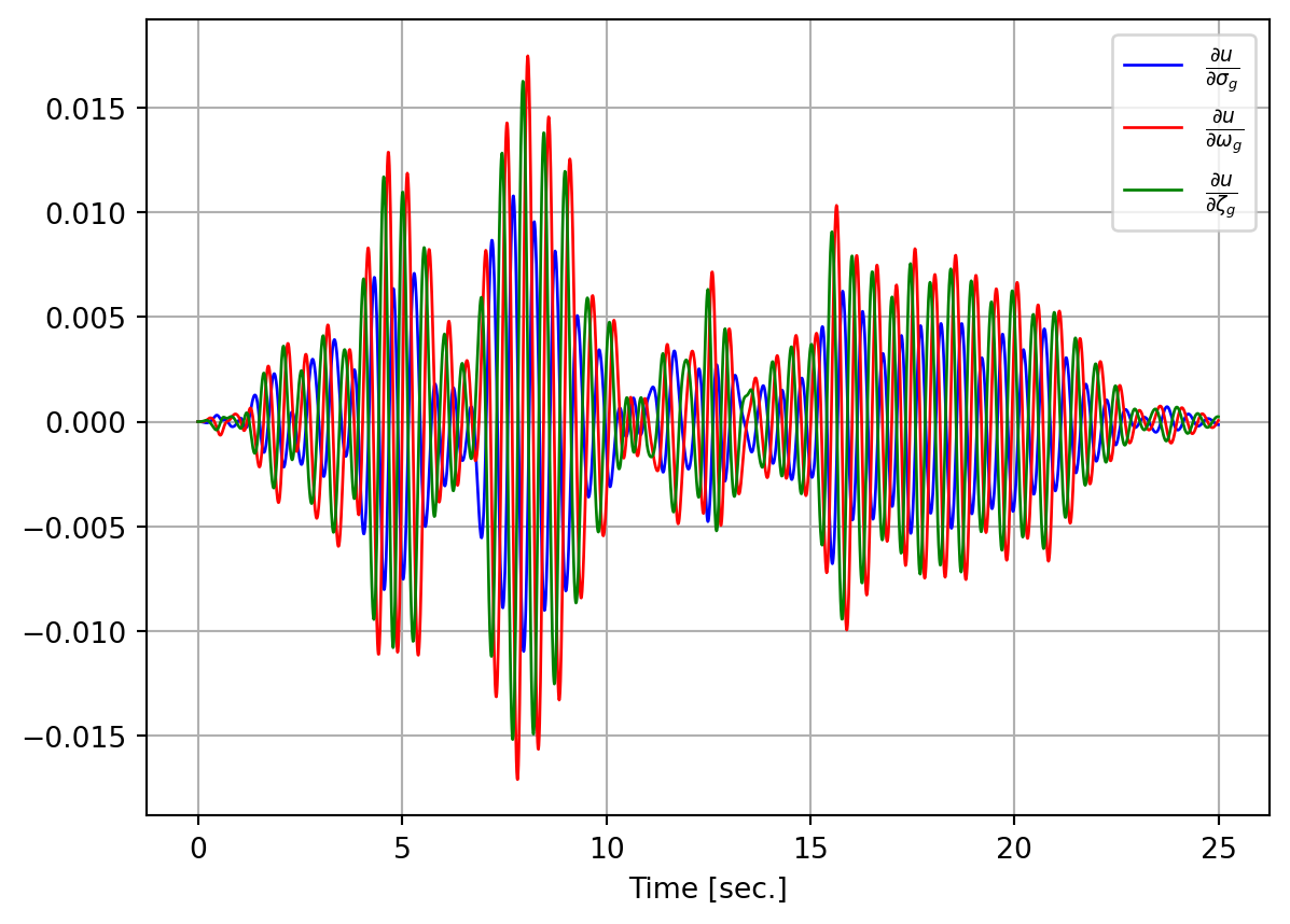
Again, we observe that \(\frac{\partial u}{\partial \sigma_g}\) seems to be more prominent for the spectral approach, while \(\frac{\partial u}{\partial \omega_g}\) appears somewhat more important for the structure subjected to the filtered white noise ground motion.