from Chapter11code import *12 Nonlinear MDOF Dynamics
At first glance, multi-DOF nonlinear dynamics appears the same as the single-DOF nonlinear dynamic analysis addressed in the previous chapter. In fact, the equation of motion in Equation 11.1 is valid for multi-DOF problems as well, as seen in Equation 1.5, only with vector and matrix symbols instead of scalars.
A distinction emerges, however, in sensitivity analysis when the damping matrix employs the current tangent stiffness matrix, updated through the iterations and increments of the analysis. That is the case either when the tangent stiffness matrix is used directly in the second term in Equation 10.18, or when the eigenvalues and eigenvectors in any of the damping models in Equation 10.17 and Equation 10.18 are calculated using the current tangent stiffness matrix.
Those are options utilized in engineering practice. In turn, that affects the sensitivity calculations in a special way, as pointed out by Haukaas (2024) and described below. The issue is specific to material models whose stiffness changes continuously with the strain. That is not the case for the bilinear material model, which is why a new material model is introduced in this chapter.
12.1 Damping Derivatives
The following damping models are identified in the paper cited above:
- MI = modal damping with eigenvalues and vectors determined once and for all using the initial stiffness matrix
- MT = modal damping with eigenvalues and vectors updated at every iteration at every increment, using the current tangent stiffness matrix
- RI = Rayleigh damping with the initial stiffness matrix appearing in the second term in Equation 10.18 and the proportionality constants \(c_M\) and \(c_K\) calculated with eigenvalues and vectors determined once and for all using the initial stiffness matrix
- RTi = Rayleigh damping with the current tangent stiffness matrix appearing in the second term in Equation 10.18 but with the proportionality constants calculated with eigenvalues and vectors determined once and for all using the initial stiffness matrix
- RTt = Rayleigh damping with the current tangent stiffness matrix appearing in the second term in Equation 10.18 and the proportionality constants \(c_M\) and \(c_K\) calculated with eigenvalues and vectors updated at every iteration at every increment, using the current tangent stiffness matrix
Any of the damping options with a “T” or “t” in the name requires a reconsideration of the damping matrix derivatives in Section 10.8. In fact, the amendment is such that it affects the coefficient matrix in the system of equations for response sensitivities. This is seen by acknowledging the implicit and potentially explicit dependence of the damping matrix on the variable \(x\), an issue described in Section 8.1.1. That point applied to the damping matrix yields
\[ \frac{\partial \mathbf{C}}{\partial x} = \frac{\partial \mathbf{C}}{\partial \mathbf{K}} \frac{\partial \mathbf{K}}{\partial \mathbf{u}} \frac{\partial \mathbf{u}_{n+1}}{\partial x} + \left. \frac{\partial \mathbf{C}}{\partial x} \right|_{\mathbf{u}_{n+1} \: \mathrm{fixed}} \tag{12.1}\]
Equation 10.42 and Equation 11.9 show that \(\frac{\partial \mathbf{C}}{\partial x}\) multiplies the parenthesis \(\left(a_5 \mathbf{u}_{n+1} + a_6 \mathbf{u}_n + a_7 \dot{\mathbf{u}}_n + a_8 \ddot{\mathbf{u}}_n \right)\), which according to Equation 10.39 is the velocity at the current time step, i.e., \(\dot{\mathbf{u}}_{n+1}\). For the second term in the right-hand side of Equation 12.1, that multiplication is trivial. In fact, the conditional derivative of the damping matrix, i.e., the second term in the right-hand side of Equation 12.1 simply takes the place of the damping derivative, in the aforementioned Equation 10.42 and Equation 11.9.
The first term in the right-hand side of Equation 12.1 requires more attention. That is because the sought response sensitivity, \(\frac{\partial \mathbf{u}_{n+1}}{\partial x}\), appears in that term. For that reason, that term needs to be moved to the left-hand side of the system of equations that governs \(\frac{\partial \mathbf{u}_{n+1}}{\partial x}\). To that end, we rewrite the left-hand side of the system of equations in Equation 10.42 and Equation 11.9 as
\[ \left(a_1 \mathbf{M} + a_5 \mathbf{C} + \mathbf{K} + \frac{\partial \mathbf{C}}{\partial \mathbf{K}} \frac{\partial \mathbf{K}}{\partial \mathbf{u}} \dot{\mathbf{u}}_{n+1} \right) \frac{\partial \mathbf{u}_{n+1}}{\partial x} = \text{right-hand side} \tag{12.2}\]
The vector-matrix notation in that equation is not well defined. Pulling \(\frac{\partial \mathbf{u}_{n+1}}{\partial x}\) outside the product \(\frac{\partial \mathbf{C}}{\partial \mathbf{K}} \frac{\partial \mathbf{K}}{\partial \mathbf{u}} \frac{\partial \mathbf{u}_{n+1}}{\partial x}\dot{\mathbf{u}}_{n+1}\) is unclear unless we employ index notation. First, the complete vector-matrix product in Equation 12.1 multiplied with the current velocity is translated into index notation as follows:
\[ \begin{aligned} \frac{\partial \mathbf{C}_{n+1}}{\partial \mathbf{K}_{n+1}} \frac{\partial \mathbf{K}_{n+1}}{\partial \mathbf{u}_{n+1}} \frac{\partial \mathbf{u}_{n+1}}{\partial x} \dot{\mathbf{u}}_{n+1} &= \frac{\partial C_{ij}}{\partial K_{op}} \frac{\partial K_{op}}{\partial u_m} \frac{\partial u_m}{\partial x} v_j \\ &= \left( \frac{\partial C_{ij}}{\partial K_{op}} \frac{\partial K_{op}}{\partial u_m} v_j \right) \frac{\partial u_m}{\partial x} \end{aligned} \tag{12.3}\]
The last parenthesis is the term that must be added to the coefficient matrix in the left-hand side of the linear system of equations, which is shown for linear dynamics in Equation 10.42. Note the following about that term:
- \(\dot{\mathbf{u}}_{n+1} \equiv \mathbf{v} \equiv v\) is introduced to simplify notation, i.e., to avoid the appearance of the increment index
- The amendment is parameter-independent, meaning that it needs to be calculated only once, regardless of how many parameters that response sensitivities are calculated with respect to
- The index of the velocity vector, \(\mathbf{v}\), contracts with the second index of the forth-order tensor \(\partial \mathbf{C} / \partial \mathbf{K}\)
- For Rayleigh damping expressed directly in terms of the tangent stiffness matrix, the fourth-order tensor \(\partial \mathbf{C} / \partial \mathbf{K}\) contains \(\partial \mathbf{K} / \partial \mathbf{K}\) , i.e., the fourth-order identity tensor. In that case, the identity tensor acts to replace the dummy indices \(op\) of \(\partial \mathbf{K} / \partial \mathbf{u}\) by \(im\), resulting in the contraction of the index of \(\mathbf{v}\) with the middle index of the third-order tensor \(\partial \mathbf{K} / \partial \mathbf{u}\)
In summary, the system of equations that governs first-order response sensitivities in nonlinear dynamics is the following generalization of Equation 11.9
\[ \begin{aligned} &\left(a_1 \mathbf{M} + a_5 \mathbf{C} + \mathbf{K} + \frac{\partial \mathbf{C}}{\partial \mathbf{K}} \frac{\partial \mathbf{K}}{\partial \mathbf{u}} \dot{\mathbf{u}}_{n+1} \right) \frac{\partial \mathbf{u}_{n+1}}{\partial x} =- \frac{\partial \mathbf{M}}{\partial x} \cdot \ddot{u}_g(t_{n+1}) \\ &- \frac{\partial \mathbf{M}}{\partial x} \left(a_1 \mathbf{u}_{n+1} + a_2 \mathbf{u}_n + a_3 \dot{\mathbf{u}}_n + a_4 \ddot{\mathbf{u}}_n \right) \\ &- \mathbf{M} \left(a_2 \frac{\partial \mathbf{u}_n}{\partial x} + a_3 \frac{\partial \dot{\mathbf{u}}_n}{\partial x} + a_4 \frac{\partial \ddot{\mathbf{u}}_n}{\partial x} \right) \\ &- \left. \frac{\partial \mathbf{C}}{\partial x} \right|_{u_{n+1} \: \mathrm{fixed}} \left(a_5 \mathbf{u}_{n+1} + a_6 \mathbf{u}_n + a_7 \dot{\mathbf{u}}_n + a_8 \ddot{\mathbf{u}}_n \right) \\ &- \mathbf{C} \left(a_6 \frac{\partial \mathbf{u}_n}{\partial x} + a_7 \frac{\partial \dot{\mathbf{u}}_n}{\partial x} + a_8 \frac{\partial \ddot{\mathbf{u}}_n}{\partial x} \right) \\ &- \left. \frac{\partial \tilde{\mathbf{F}}}{\partial x} \right|_{u_{n+1} \: \mathrm{fixed}} \end{aligned} \tag{12.4}\]
The quantities \(\frac{\partial \mathbf{C}}{\partial \mathbf{K}}\) and \(\frac{\partial \mathbf{K}}{\partial \mathbf{u}}\) are addressed in the next two sections.
12.2 New Eigen Derivatives
The conditional derivative \(\left. \frac{\partial \mathbf{C}}{\partial x} \right|_{u_{n+1} \: \mathrm{fixed}}\) that appears in Equation 12.4 is given in Section 10.8, for modal and Rayleigh damping. However, the quantity \(\frac{\partial \mathbf{C}}{\partial \mathbf{K}}\) is new in this chapter. Using index notation and the symbol \(m \equiv M_n\) for modal mass and \(\omega \equiv \omega_n\) for natural frequency, that derivative is, for the modal damping model:
\[ \frac{\partial C_{ik}}{\partial K_{op}} = \frac{\partial C_{ik}}{\partial m} \frac{\partial m}{\partial \phi_q} \frac{\partial \phi_q}{\partial K_{op}} + \frac{\partial C_{ik}}{\partial \omega} \frac{\partial \omega}{\partial K_{op}} + \frac{\partial C_{ik}}{\partial \phi_q} \frac{\partial \phi_q}{\partial K_{op}} \tag{12.5}\]
For Rayleigh damping, the derivative is
\[ \begin{aligned} \frac{\partial C_{ij}}{\partial K_{op}} &= \frac{\partial \check{\omega}}{\partial K_{op}}\cdot \frac{2 \zeta \cdot \hat{\omega}}{\check{\omega} + \hat{\omega}} \cdot M_{ij} + \frac{\partial \hat{\omega}}{\partial K_{op}}\cdot \frac{2 \zeta \cdot \check{\omega}}{\check{\omega} + \hat{\omega}} \cdot M_{ij} \\ &- \frac{2 \zeta \cdot \check{\omega} \cdot \hat{\omega}}{(\check{\omega} + \hat{\omega})^2} \left( \frac{\partial \check{\omega}}{\partial K_{op}}+\frac{\partial \hat{\omega}}{\partial K_{op}}\right) M_{ij} \\ &- \frac{2 \zeta}{(\check{\omega} + \hat{\omega})^2} \left( \frac{\partial \check{\omega}}{\partial K_{op}}+\frac{\partial \hat{\omega}}{\partial K_{op}}\right) K_{ij} + \frac{2 \zeta}{\check{\omega} + \hat{\omega}} \cdot \frac{\partial K_{ij}}{\partial K_{op}} \end{aligned} \tag{12.6}\]
where \(\partial K_{ij} / \partial K_{op}\) in the last term is the fourth-order identity tensor mentioned earlier. Those equations show that derivatives of natural frequencies and eigenvectors with respect to the stiffness matrix are needed. To that end, differentiation of Equation 10.31 gives
\[ \left( \frac{\partial K_{ij}}{\partial K_{kl}} - \frac{\partial \gamma}{\partial K_{kl}} M_{ij} - \gamma \frac{\partial M_{ij}}{\partial K_{kl}} \right) \phi_j + \left( K_{ij} - \gamma M_{ij} \right) \frac{\partial \phi_j}{\partial K_{kl}} = 0_i \tag{12.7}\]
Multiplying through by \(\phi_i\) causes the last term to vanish, as earlier, leading to
\[ \phi_i \frac{\partial K_{ij}}{\partial K_{kl}} \phi_j - \phi_i \frac{\partial \gamma}{\partial K_{kl}} M_{ij} \phi_j - \phi_i \gamma \frac{\partial M_{ij}}{\partial K_{kl}} \phi_j = 0 \tag{12.8}\]
Again, it is assumed that the derivative of mass with respect to stiffness is zero, effectively removing the last term. Also, the first term simplifies because \(\partial K_{ij} / \partial K_{kl}\) is the identity tensor. As a result, the first term is the outer product \(\phi_k \phi_l\), leading to the eigenvalue derivative
\[ \frac{\partial \gamma}{\partial K_{kl}} = \frac{\phi_k \phi_l}{\phi_i M_{ij} \phi_j} \tag{12.9}\]
Equation 12.7 gives the corresponding eigenvector derivative, employing the pseudo-inverse, as was done in Chapter 10:
\[ \frac{\partial \phi_j}{\partial K_{kl}} = -\left( K_{ij} - \gamma M_{ij} \right)^+ \left( \frac{\partial K_{ij}}{\partial K_{kl}} - \frac{\partial \gamma}{\partial K_{kl}} M_{ij} \right) \phi_j \tag{12.10}\]
Those derivatives are calculated by the following function:
def eigenDerivativesWrtK(K, M, gammas, vectors):
    dgammasdK = []
    domegasdK = []
    dvectorsdK = []
    for mode in range(len(gammas)):
        lhs = (vectors[mode].dot(M)).dot(vectors[mode])
        rhs = np.outer(vectors[mode], vectors[mode])
        gammaDerivative = rhs / lhs
        dgammasdK.append(gammaDerivative)
        domegasdK.append(0.5 / np.sqrt(gammas[mode]) * gammaDerivative)
        pseudoInverse = np.linalg.pinv(np.subtract(K, np.multiply(gammas[mode], M)))
        gammaTimesM = np.einsum('kl,ij->klij', gammaDerivative, M)
        dKdK = np.einsum('ik,jl->ijkl', np.eye(len(K)), np.eye(len(K)))
        onedvectordK = np.einsum('pi,klij,j->pkl', pseudoInverse, (gammaTimesM - dKdK), vectors[mode])
        dvectorsdK.append(onedvectordK)
    return dgammasdK, domegasdK, dvectorsdK
12.3 Bouc-Wen Material
The derivative \(\partial \mathbf{K} / \partial \mathbf{u}\) that appears in Equation 12.4 is usually not calculated in structural analysis. It is non-zero only for material models whose stiffness changes continuously with strain. When piece-wise linear constitutive relationships are used, i.e., when the bilinear material model employed previously in this book is utilized, then the stiffness does not vary continuously with the strain. In that case, the coefficient matrix for the first-order response sensitivity calculations is the ordinary effective dynamic stiffness that appears in Equation 10.42. In other words, when piece-wise linear constitutive relationships are used, then \(\frac{\partial \mathbf{K}}{\partial \mathbf{u}} = \mathbf{0}\) and the last term in the parenthesis in the left-hand side of Equation 12.4 vanishes. In that case, the treatment of damping is identical to Chapter 10. A material model that does exhibit continuous variation of stiffness with strain is the Bouc-Wen model. It expresses the stress at time \(t_{n+1}\) as a sum of an elastic total-strain portion and a hysteretic part based on incremental strain:
\[ \sigma_{n+1} = \alpha \cdot E \cdot \varepsilon_{n+1} + (1-\alpha) \cdot f_y \cdot z_{n+1} \tag{12.11}\]
\(z\) is an auxiliary hysteretic evolution variable governed by the differential equation
\[ \dot{z} = \left( \dot{\varepsilon} - \gamma \cdot \dot{\varepsilon} \cdot |z|^\eta - \beta \cdot |\dot{\varepsilon}| \cdot z^\eta \right) \cdot \frac{1}{\varepsilon_y} = \left( 1 - \left( \gamma + \beta \cdot \text{sgn} \left (\dot{\varepsilon} \cdot z \right) \right) \cdot |z|^\eta \right) \frac{\dot{\varepsilon}}{\varepsilon_y} \tag{12.12}\]
where values for \(\gamma\), \(\beta\), and \(\eta\) are addressed in the next section and, in the last equality, \(\dot{\varepsilon}\) and \(|z|^\eta\) are pulled outside the parentheses, resulting in the shown use of the signum function. As a result of that rearrangement, the analytical version of the derivative \(\partial z / \partial \varepsilon\), employed shortly, is available as the term in the outermost parentheses in Equation 12.12) if divided by \(\varepsilon_y\). That fact is understood by observing the chain rule of differentiation in the form \(\dot{z} \equiv \partial z / \partial t = (\partial z / \partial \varepsilon)(\partial \varepsilon / \partial t) \equiv (\partial z / \partial \varepsilon) \dot{\varepsilon}\) and comparing that result with the last equality in Equation 12.12. Next, by setting \(\dot{\varepsilon}=(\varepsilon_{n+1}-\varepsilon_n)/ \Delta t\), the Backward Euler scheme for solving Equation 12.12 is, once \(\Delta t\) cancels,
\[ z_{n+1} = z_n + \left( 1 - \left( \gamma + \beta \cdot \text{sgn}(\dot{\varepsilon}_{n+1} \cdot z_n) \right) \cdot |z_{n+1}|^\eta \right) \cdot \frac{\varepsilon_{n+1}-\varepsilon_n}{\varepsilon_y} \tag{12.13}\]
where \(\text{sgn}(\dot{\varepsilon}_{n+1} \cdot z_n)\) is employed instead of \(\text{sgn}(\dot{\varepsilon}_{n+1} \cdot z_{n+1})\) in order to detect load reversals in a consistent manner, i.e., to avoid spurious load reversals during the Newton-Raphson iterations. The unknown \(z_{n+1}\) appears on both sides of Equation 12.13; it is determined by the iterative Newton algorithm. For this material model, four quantities are derived and implemented in this paper for the purpose of response sensitivity calculations: The algorithmically consistent tangent stiffness \(\partial \sigma_{n+1} / \partial \varepsilon_{n+1}\); the conditional stress derivative \(\partial \sigma_{n+1} / \partial x\); the conditional stiffness derivative \(\partial k_{n+1} / \partial x\); and the unconditional stiffness derivative \(\partial k_{n+1} / \partial \varepsilon_{n+1}\) for the third-order tensor that appeared earlier. Differentiation of the stress in Equation 12.11 with respect to the strain gives the algorithmic tangent modulus
\[ k_{n+1} = \frac{\partial \sigma_{n+1}}{\partial \varepsilon_{n+1}} = \alpha \cdot E + (1-\alpha) \cdot f_y \cdot \frac{\partial z_{n+1}}{\partial \varepsilon_{n+1}} \tag{12.14}\]
The algorithmically consistent material tangent modulus is obtained by substituting the algorithmically consistent version of the derivative \(\partial z_{n+1} / \partial \varepsilon_{n+1}\). That means differentiating the algorithm that calculates \(z_{n+1}\), instead of utilizing the analytical version mentioned below Equation 12.12. Differentiation of Equation 12.13 with respect to \(\varepsilon_{n+1}\) and solving for \(\partial z_{n+1} / \partial \varepsilon_{n+1}\) yields
\[ \frac{\partial z_{n+1}}{\partial \varepsilon_{n+1}} = \frac{\left( 1 - \left( \gamma + \beta \cdot \text{sgn}(\dot{\varepsilon} \cdot z \right) \cdot |z|^\eta \right) \frac{1}{\varepsilon_y}}{1+\left( 1 - \left( \gamma + \beta \cdot \text{sgn}(\dot{\varepsilon} \cdot z \right) \cdot \eta \cdot |z|^{\eta-1} \cdot \text{sgn}(z) \right) \frac{1}{\varepsilon_y}} \tag{12.15}\]
where the subscript \(n+1\) is omitted for brevity on the right-hand side, and the derivative of an absolute value, i.e., \(\partial |z| / \partial x = \partial \left( \text{sgn}(z) \cdot z \right) / \partial x = \text{sgn}(z) \cdot \partial z / \partial x\), is employed here and elsewhere in this paper. Next, the derivative of the stress with respect to \(x\) is, from Eq. (33),
\[ \begin{aligned} \frac{\partial \sigma_{n+1}}{\partial x} \Big|_{\varepsilon_{n+1}\text{ fixed}} &= \frac{\partial \alpha}{\partial x} \cdot E \cdot \varepsilon_{n+1} + \alpha \cdot \frac{\partial E}{\partial x} \cdot \varepsilon_{n+1} - \frac{\partial \alpha}{\partial x} \cdot f_y \cdot z_{n+1} \\ &+ (1-\alpha) \cdot \frac{\partial f_y}{\partial x} \cdot z_{n+1} + (1-\alpha) \cdot f_y \cdot \frac{\partial z_{n+1}}{\partial x}\Big|_{\varepsilon_{n+1}\text{ fixed}} \end{aligned} \tag{12.16}\]
where the derivative of \(z\) is obtained by differentiating Equation 12.13 with respect to \(x\) and solving for \(\partial z_{n+1} / \partial x\):
\[ \frac{\partial z_{n+1}}{\partial x}\Big|_{\varepsilon_{n+1}\text{ fixed}} = \frac{|z_{n+1}| \left(\varepsilon_y \left(-b \cdot c \cdot |z_{n+1}|^{\eta }+c+\frac{\partial z_n}{\partial x} \cdot \varepsilon_y\right)- (\varepsilon_n-\varepsilon_{n+1}) \cdot \left(b \cdot |z_{n+1}|^{\eta }-1\right)\right)}{\varepsilon_y \cdot \left(\varepsilon_y \cdot |z_{n+1}|- a \cdot b \cdot \eta \cdot (\varepsilon_n-\varepsilon_{n+1}) \cdot |z_{n+1}|^{\eta }\right)} \tag{12.17}\]
The following symbols are introduced to abbreviate that expression:
\[ a = \text{sgn}(z_{n+1}) \;\;\;\;\;\;\;\; b = \gamma + \beta \cdot \text{sgn}(\dot{\varepsilon}_{n+1} \cdot z_n) \;\;\;\;\;\;\;\; c = \frac{\partial \varepsilon_{n+1}}{\partial x} - \frac{\partial \varepsilon_n}{\partial x} \tag{12.18}\]
It is noted that \(\partial z_n / \partial x\) appears in Equation 12.17, implying that the unconditional derivative of \(\partial z_{n+1} / \partial x\) must be calculated and stored once the response sensitivities are calculated. Specifically, in the factor \(c\) in Equation 12.18, the quantity \(\partial \varepsilon_{n+1} / \partial x\) is zero when conditional derivatives are calculated and non-zero when unconditional derivatives are saved, obtained from the response sensitivity \(\partial \mathbf{u}_{n+1} / \partial x\). Next, the derivative of the stiffness with respect to \(x\) is obtained by differentiating Equation 12.14:
\[ \begin{aligned} \frac{\partial k_{n+1}}{\partial x} \Big|_{\varepsilon_{n+1}\text{ fixed}} &= \frac{\partial \alpha}{\partial x} \cdot E + \alpha \cdot \frac{\partial E}{\partial x} - \frac{\partial \alpha}{\partial x} \cdot f_y \cdot \frac{\partial z_{n+1}}{\partial \varepsilon_{n+1}} \\ &+ (1-\alpha) \cdot \frac{\partial f_y}{\partial x} \cdot \frac{\partial z_{n+1}}{\partial \varepsilon_{n+1}} + (1-\alpha) \cdot f_y \cdot \frac{\partial^2 z_{n+1}}{\partial \varepsilon_{n+1} \partial x}\Big|_{\varepsilon_{n+1}\text{ fixed}} \end{aligned} \tag{12.19}\]
Here, the double-derivative of \(z\) is obtained by first differentiating Equation 12.13 with respect to the current strain, done above in order to obtain the stiffness, then differentiating with respect to \(x\), making it possible to solve for the result
\[ \frac{\partial^2 z_{n+1}}{\partial \varepsilon_{n+1} \partial x}\Big|_{\varepsilon_{n+1}\text{ fixed}} = \frac{b \cdot |z_{n+1}|^{\eta } \left(a \cdot d \cdot \varepsilon_y \cdot \eta+ |z_{n+1}| \left(\frac{\partial z_{n+1}}{\partial \varepsilon_{n+1}} \cdot a \cdot \eta \cdot (\varepsilon_{n+1}-\varepsilon_n)+|z_{n+1}| \right) \right)- |z_{n+1}|^2}{\varepsilon_y \cdot |z_{n+1}| \cdot \left(\varepsilon_y \cdot |z_{n+1}|-\eta \cdot a \cdot b \cdot (\varepsilon_n-\varepsilon_{n+1}) \cdot |z_{n+1}|^{\eta }\right)} \tag{12.20}\]
where the auxiliary variable
\[ d = a \cdot \frac{\partial z_{n+1}}{\partial \varepsilon_{n+1}} \frac{\partial z_{n+1}}{\partial x} (\eta -1) (\varepsilon_n-\varepsilon_{n+1})-|z_{n+1}| \left(\frac{\partial \varepsilon_{n+1}}{\partial x} \frac{\partial z_{n+1}}{\partial \varepsilon_{n+1}}-\frac{\partial \varepsilon_n}{\partial x} \frac{\partial z_{n+1}}{\partial \varepsilon_{n+1}}+\frac{\partial z_{n+1}}{\partial x} \right) \tag{12.21}\]
is defined. Notice that no other derivative at time \(t_n\) than \(\partial z_n / \partial x\) and \(\partial \varepsilon_n / \partial x\) appear; only those two quantities need to be stored. Finally, the derivative of the stiffness with respect to the strain is obtained by first differentiating Equation 12.14, which yields
\[ \frac{\partial k_{n+1}}{\partial \varepsilon_{n+1}} = (1-\alpha) \cdot f_y \cdot \frac{\partial^2 z_{n+1}}{\partial \varepsilon_{n+1}^2} \tag{12.22}\]
The double-derivative of \(z\) in Equation 12.22 is obtained by differentiating Equation 12.13 twice with respect to the current strain and solving for
\[ \frac{\partial^2 z_{n+1}}{\partial \varepsilon_{n+1}^2} = \frac{a \cdot b \cdot \eta \cdot \frac{\partial z_{n+1}}{\partial \varepsilon_{n+1}} \cdot (2 \cdot |z_{n+1}|-a \cdot \frac{\partial z_{n+1}}{\partial \varepsilon_{n+1}} \cdot (\eta -1) \cdot (\varepsilon_n-\varepsilon_{n+1}))}{a \cdot b \cdot \eta \cdot |z_{n+1}| \cdot (\varepsilon_n-\varepsilon_{n+1})-\varepsilon_y \cdot |z_{n+1}|^{2-\eta }} \tag{12.23}\]
The complete code for the Bouc-Wen material model, with functions that implement the equations derived above, is made available in Appendix D and imported here:
from AppendixDcode import *12.4 Analysis Algorithm
The algorithm that solves Equation 1.5 for \(\mathbf{u}\) and Equation 12.4 for \(\frac{\partial \mathbf{u}}{\partial x}\) is too large to be neatly present here. It is provided in Appendix E and imported here:
from AppendixEcode import *Although that code is large, some comment lines are provided to help descipher it. A novelty of that code is the Kamendment matrix, which amends the effective tangent stiffness before first-order sensitivities are calculated with the command np.linalg.solve(ddmKeffective, ddmRHSf), where ddmRHSf is the right-hand side of Equation 12.4 in the final structural DOF configuration. Returned from that analysis algorithm are ten items:
tis the time axisgroundAccelerationis the ground accelerationuTrackcontains the displacement at the tracked nodes and DOFsvTrackcontains the velocity at the tracked nodes and DOFsaTrackcontains the acceleration at the tracked nodes and DOFsdudxcontains the first-order sensitivity of the displacementsdvdxcontains the first-order sensitivity of the velocitiesdadxcontains the first-order sensitivity of the accelerationsdnl1is a “degree of nonlinearity” defined as the ratio of the initial first natural frequency to the current natural frequencydnl2is the same for the second natural frequency
When extracting responses, use the format uTrack[which-tracked-u, which-time]. When extracting response sensitivities, use the format dudx: [which-tracked-u, which-variable, which-time]. This is exemplified next.
12.5 Column Example
A column like that analyzed in Chapter 10 is used as an example in this chapter, only now the behaviour is nonlinear and modelled with the Boud-Wen material:
def createNonlinearColumnInput(E, fy, alpha, hw, bf, tf, tw, rho, nel):
    L = 15
    A = tw*(hw-2*tf) + 2*bf*tf
    M = A * L/nel * rho
    q = 0
    nf = 2      # Number of fibers in the flange
    nw = 8      # Number of fibres in the web
    nsec = 5    # Number of integration points
    eta = 3     # Bouc-Wen sharpness
    gamma = 0.5 # Bouc-Wen parameter
    beta = 0.5  # Bouc-Wen parameter
    NODES = []
    for i in range(nel+1):
        NODES.append([0.0, i*L/nel])
    CONSTRAINTS = [[1, 1, 1]]
    for i in range(nel):
        CONSTRAINTS.append([0, 0, 0])
    ELEMENTS = []
    SECTIONS = []
    MATERIALS = []
    for i in range(nel):
        ELEMENTS.append([12, nsec, q, i+1, i+2])
        SECTIONS.append(['WideFlange', hw, bf, tf, tw, nf, nw])
        MATERIALS.append(['BoucWen', E, fy, alpha, eta, beta, gamma])
        #MATERIALS.append(['Bilinear', E, fy, alpha])
    LOADS = np.zeros((nel+1, 3))
    MASS = [[0, 0, 0]]
    for i in range(nel-1):
        MASS.append([M, 0, 0])
    MASS.append([0.5*M, 0, 0])
    input = [NODES, CONSTRAINTS, ELEMENTS, SECTIONS, MATERIALS, LOADS, MASS]
    return input
The variables with respect to which response sensitivities are calculated are defined in the DDMs array in the following function:
def nonlinearColumnVariableSpecs(nel):
    E = 200e9     # Initial stiffness, N/m^2
    fy = 350e6    # Yield stress, N/m^2
    alpha = 0.05  # Second-slope stiffness coefficient
    hw = 0.350    # Web height, m (W360X147 = W14x99)
    bf = 0.370    # Flange width, m
    tf = 0.0198   # Flange thickness, m
    tw = 0.0123   # Web thickness, m
    rho = 7850.0  # kg/m^3
    means = [E, fy, alpha, hw,   bf,   tf,   tw,   rho]
    covs = [0.1, 0.2, 0.2, 0.05, 0.05, 0.05, 0.05, 0.05]
    stdvs = np.array(means) *np.array(covs)
    correlation = []
    distributions = []
    dM = [[0, 0, 0]]
    for i in range(nel-1):
        dM.append([1, 0, 0])
    dM.append([0.5, 0, 0])
    DDMs = [['Element', 'E', range(1, nel+1)],
            ['Element', 'fy', range(1, nel+1)],
            ['Element', 'alpha', range(1, nel+1)],
            ['Element', 'hw', range(1, nel+1)],
            ['Element', 'bf', range(1, nel+1)],
            ['Element', 'tf', range(1, nel+1)],
            ['Element', 'tw', range(1, nel+1)],
            ['Node', 'M', dM],
            ['Model', 'targetDamping']]
    trackNode = [nel+1]
    trackDOF = [1]
    return means, stdvs, distributions, correlation, trackNode, trackDOF, DDMs
Here is a plot of the structural model:
nel = 5
means, stdvs, distributions, correlation, trackNode, trackDOF, DDMs = nonlinearColumnVariableSpecs(nel)
input = createNonlinearColumnInput(*means, nel)
structuralModel = model(input)
structuralModel.plotModel()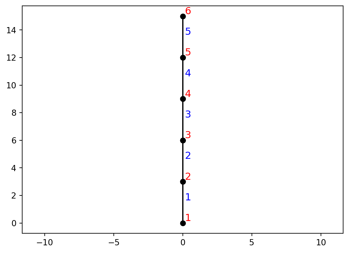
The damping models listed at the start of this chapter are all viable options in the analysis:
targetDamping = 0.05
dampingMI = ['Modal', 'Initial', targetDamping]
dampingMT = ['Modal', 'Current', targetDamping]
dampingRI = ['Rayleigh', 'Initial', 'Initial', 1, 2, targetDamping]
dampingRTi = ['Rayleigh', 'Current', 'Initial', 1, 2, targetDamping]
dampingRTt = ['Rayleigh', 'Current', 'Current', 1, 2, targetDamping]
Instead of utilizing the El Centro ground motion, a half sine wave is used as ground motion, defined below. This is done to reduce computation time and ease the interpretation of the results. A plot of the ground motion is provided below this definition:
dt = 0.02
t = np.arange(0, 2, dt)
groundAcceleration = np.zeros(len(t))
for i in range(len(t)):
    if t[i] <= 0.5:
        groundAcceleration[i] = 5 * 9.81 * np.sin(2 * np.pi * t[i])
gmMatrix = np.concatenate(([t], [groundAcceleration]), axis=0)
plt.figure()
plt.plot(gmMatrix[0], gmMatrix[1], 'k-', linewidth=1.0)
plt.xlabel("Time [sec.]")
plt.ylabel("Ground Acceleration [$\\frac{m}{s^2}$]")
plt.grid(True)
plt.show()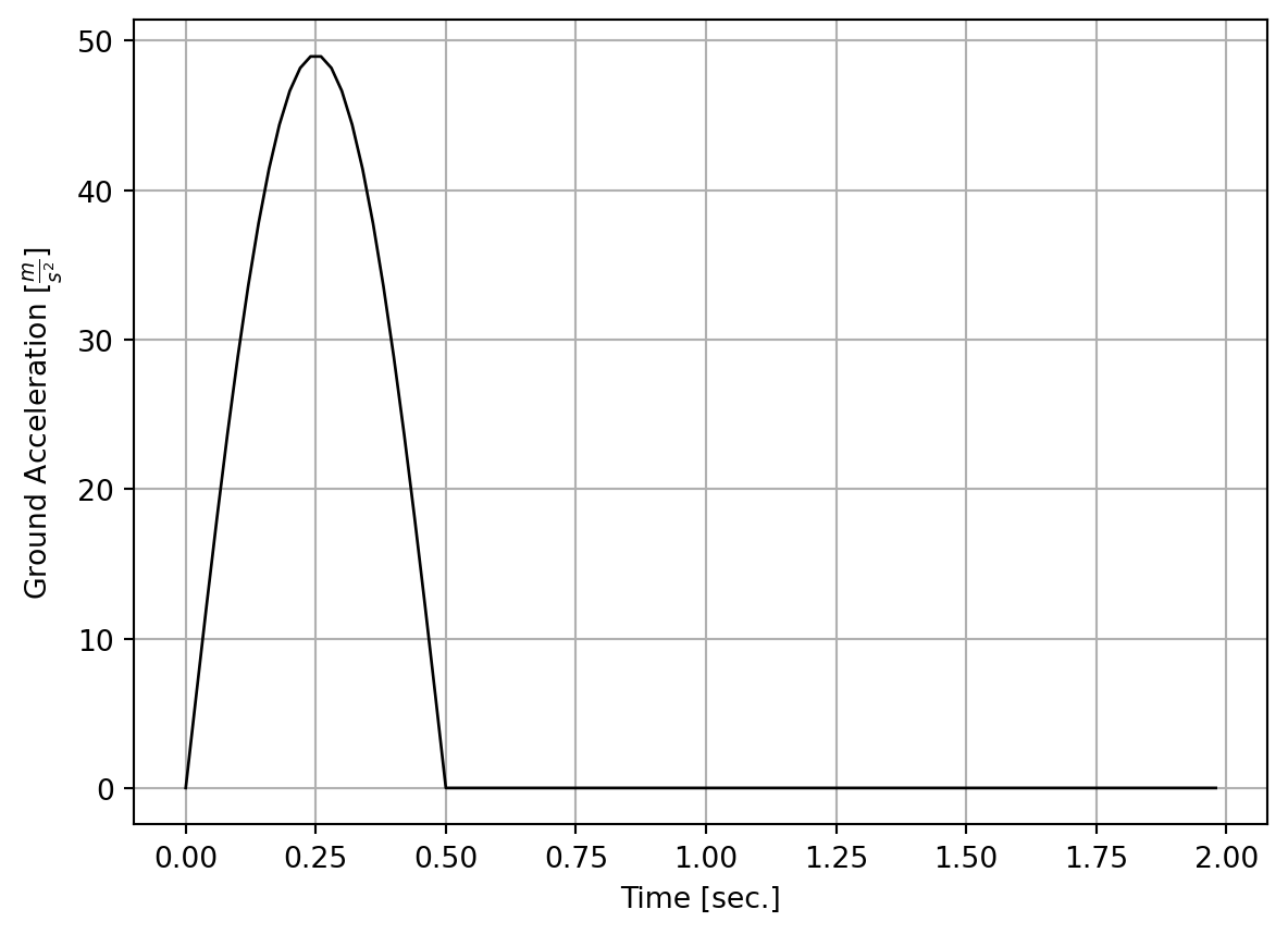
Next, the structural analysis is run, with damping model specified in the second argument. If you try different damping models, consider reducing the dt variable defined above, to ensure convergence of the Newton-Raphson algorithm, which is run here:
t, gm, u, v, a, dudx, dvdx, dadx, dnl1, dnl2 = nonlinearDynamicAnalysis(structuralModel, dampingMI, gmMatrix, trackNode, trackDOF, 1, DDMs)A plot of the displacement response at the top of of the column, and its response sensitivities, is provided below:
plt.figure()
uLabelSet = False
for i in range(1, len(t)):
    if dnl1[i] > 1.2:
        plt.plot([t[i-1], t[i]], [u[0, i-1], u[0, i]], 'r-', linewidth=1.0)
    elif dnl1[i] > 1.05:
        plt.plot([t[i-1], t[i]], [u[0, i-1], u[0, i]], 'm-', linewidth=1.0)
    else:
        if uLabelSet:
            plt.plot([t[i-1], t[i]], [u[0, i-1], u[0, i]], 'k-', linewidth=1.0)
        else:
            plt.plot([t[i-1], t[i]], [u[0, i-1], u[0, i]], 'k-', linewidth=1.0, label='u')
            uLabelSet = True
plt.plot(t, dudx[0, 0, :]*stdvs[0], 'b-', linewidth=1.0, label='$\\frac{\\partial u}{\\partial E}$')
plt.plot(t, dudx[0, 1, :]*stdvs[1], 'r-', linewidth=1.0, label='$\\frac{\\partial u}{\\partial f_y}$')
plt.plot(t, dudx[0, 2, :]*stdvs[2], 'g-', linewidth=1.0, label='$\\frac{\\partial u}{\\partial \\alpha}$')
plt.plot(t, dudx[0, 3, :]*stdvs[3], 'c-', linewidth=1.0, label='$\\frac{\\partial u}{\\partial h_w}$')
plt.plot(t, dudx[0, 4, :]*stdvs[4], 'm-', linewidth=1.0, label='$\\frac{\\partial u}{\\partial b_f}$')
plt.plot(t, dudx[0, 5, :]*stdvs[5], 'y-', linewidth=1.0, label='$\\frac{\\partial u}{\\partial t_f}$')
plt.plot(t, dudx[0, 6, :]*stdvs[6], 'g--', linewidth=1.0, label='$\\frac{\\partial u}{\\partial t_w}$')
hw = means[3]; bf = means[4]; tf = means[5]; tw = means[6]
A = tw*(hw-2*tf) + 2*bf*tf
L = 15
plt.plot(t, dudx[0, 7, :]*A*L/nel*stdvs[7], 'm--', linewidth=1.0, label='$\\frac{\\partial u}{\\partial M}$')
plt.plot(t, dudx[0, 8, :]*0.1*targetDamping, 'c--', linewidth=1.0, label='$\\frac{\\partial u}{\\partial \\zeta}$')
plt.xlabel("Time [sec.]")
plt.legend(loc='upper right')
plt.grid(True)
plt.show()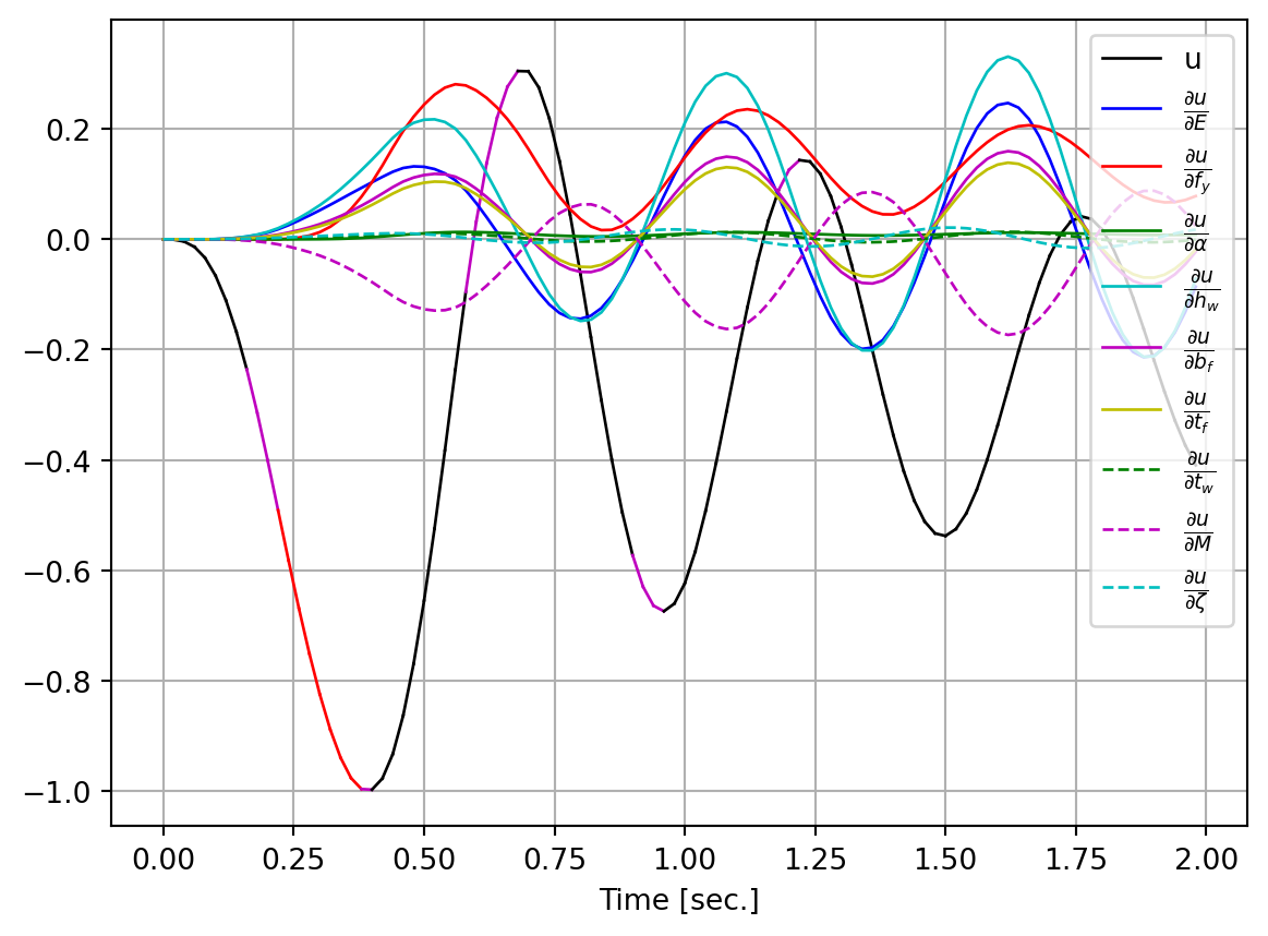
A non-black line for the displacement response indicates significant yielding, i.e., a current first natural frequency substantially different from the initial first natural frequency. Keep in mind that the Bouc-Wen material model has some degree of nonlinearity from the start. That is why a magenta coloured line is used when the natural frequency ratio is above 1.05, with a red line for ratios above 1.2. Significant yielding is observed for the ground motion specified above. As in earlier chapters, the sensitivities are normalized using the standard deviation of each variable. The coefficients of variation are provided in Listing 12.3. We note that the displacement appears quite sensitive to the yield stress, with cross-section height, \(h_w\), and mass, \(M\), following close behind.