from Chapter6code import *7 System Reliability
A system, in the context of reliability analysis, means that failure is defined by more than one limit-state function. Parallel systems is one example. In such systems, all limit-state functions must be negative before the system is considered to have failed. However, it is series systems that are of interest to structural engineers. If any limit-state is violated, the overall design is considered unsatisfactory. Each individual limit-state is referred to as a component reliability problem; such problems are addressed in the previous two chapters.
Series systems without correlation between the limit-state functions are easy to analyze and dangerous to be around. In fact, if such a system consists of many limit-states, then failure can become nearly certain, at least if the reliability index for each limit-state is low. To demonstrate this, we utilize rules of set theory and probability theory:
\[ \begin{aligned} p_{f, \mathrm{series}} &= \mathrm{P}\left(\bigcup_{k=1}^{K} g_k \leq 0 \right) \\ &= 1 - \mathrm{P}\left(\overline{\bigcup_{k=1}^{K} g_k \leq 0 }\right) \\ &= 1 - \mathrm{P}\left(\bigcap_{k=1}^{K} \overline{g_k \leq 0} \right) \\ &= 1 - \left(1-p_{f_1}\right)\cdot\left(1-p_{f_2}\right)\cdot\left(1-p_{f_3}\right)\cdots \end{aligned} \tag{7.1}\]
You can visit the website linked at the top of this page to learn more about the rules and symbols that were used:
- The first equality in Equation 7.1 employs the union symbol of set theory to define a series system
- The second equality employs the rule called probability of the complement
- The third equality employs the of de Morgan that says the complement of a union equals the intersection of complements
- The fourth equality employs the probability of the complement again to say that the probability of not violating a limit-state is one minus the probability of failure for that limit-state
The following code evaluates Equation 7.1 for several values of the reliability index and a varying number of limit-state functions. In each line of the plot, the reliability index is the same for all limit-states in the series system:
from scipy.stats import norm
plt.figure()
pBeta2 = norm.cdf(-2, 0, 1)
pBeta3 = norm.cdf(-3, 0, 1)
pBeta4 = norm.cdf(-4, 0, 1)
numComponents = []
pfForBeta2 = []
pfForBeta3 = []
pfForBeta4 = []
for k in range(2, 50):
    numComponents.append(k)
    pfForBeta2.append(1.0 - (1 - pBeta2)**k)
    pfForBeta3.append(1.0 - (1 - pBeta3)**k)
    pfForBeta4.append(1.0 - (1 - pBeta4)**k)
plt.plot(numComponents, pfForBeta2, 'k-', label='$\\beta=2$')
plt.plot(numComponents, pfForBeta3, 'b-', label='$\\beta=3$')
plt.plot(numComponents, pfForBeta4, 'r-', label='$\\beta=4$')
plt.xlabel('Number of limit-state functions')
plt.ylabel('Failure probability')
plt.grid(True)
plt.legend()
plt.show()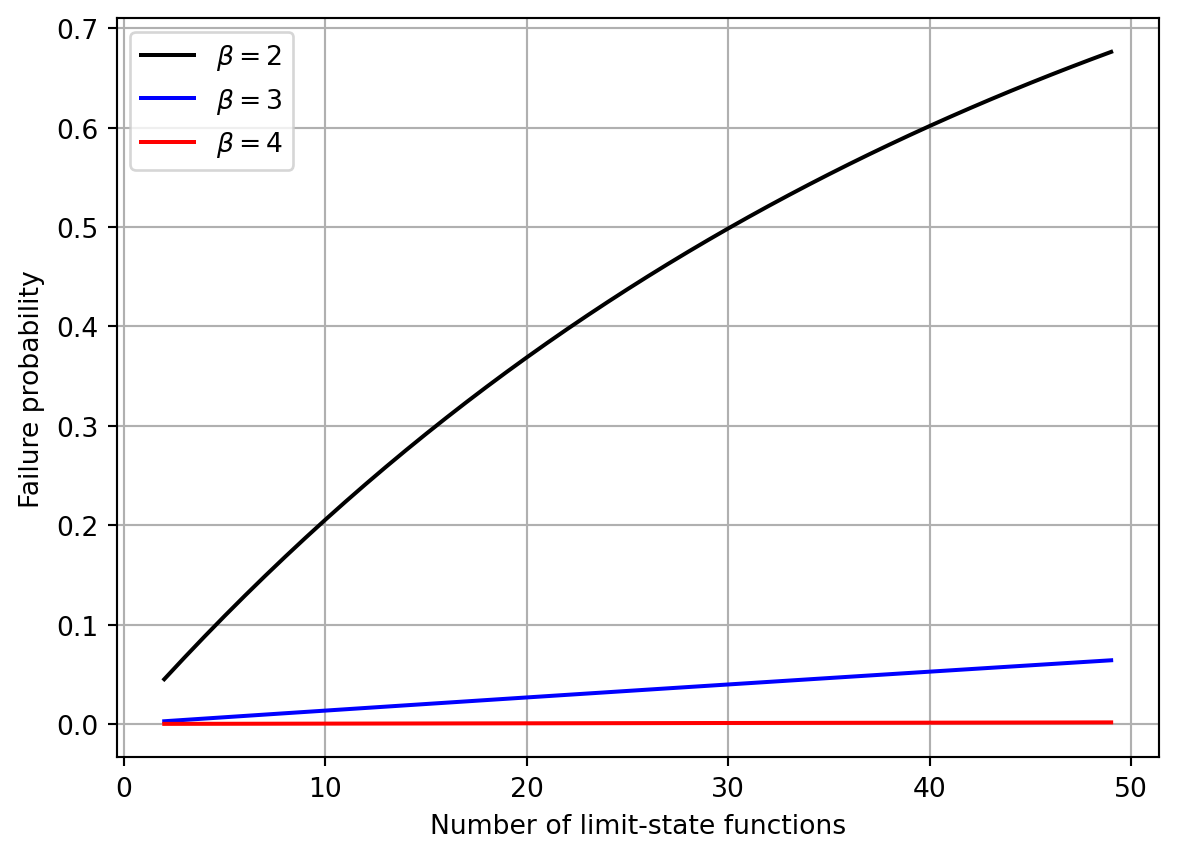
The black line in the plot shows that a reliability index as low as \(\beta=2\) for all limit-states in a series system gives a 50% chance of failure when the number of limit-states reaches 30.
7.1 Bounds for Series Systems
As will be seen later in this chapter, limit-states for structural responses are correlated. That provides safety compared with the plot shown above. However, series systems with correlated components are harder to analyze. From probability theory, it is the inclusion-exclusion rule that applies to the union of failure events in a series system. Denoting the failure event for each limit-state by \(E_k \equiv g_k(\mathbf{x}) \leq 0\) that probability rule reads
\[ \begin{aligned} p_{f, \mathrm{series}} &= \mathrm{P}\left(\bigcup_{k=1}^{K} E_k \right) \\ &= E_1 + E_2 + E_3 + \cdots \\ &= E_1 E_2 + E_1 E_3 + E_2 E_3 + \cdots \\ &= E_1 E_2 E_3 + \cdots \end{aligned} \tag{7.2}\]
Evaluating intersection probabilities like \(E_1 E_2\) and \(E_1 E_2 E_3\) is difficult for more than two limit-state functions. That point can be made in another way. Consider the series system problem expressed in the Standard Normal space:
\[ p_{f, \mathrm{series}} = \mathrm{P}\left(\bigcup_{k=1}^{K} G_k(\mathbf{y}) \leq 0 \right) \tag{7.3}\]
Next, assume that the design point, \(\mathbf{y}^*\), and the corresponding reliability index, \(\beta\), are determined for each limit-state function, with methods described in the previous two chapters. To that end, we spell out the linearization of the limit-state functions at their respective design points:
\[ \begin{aligned} G(\mathbf{y}) &\approx G(\mathbf{y}^*) + \nabla G(\mathbf{y}^*)^{\top} (\mathbf{y}-\mathbf{y}^*) \\ &= 0 - \lVert G(\mathbf{y}^*) \rVert \pmb{\alpha}^{\top}(\mathbf{y}-\mathbf{y}^*) \\ &= \lVert G(\mathbf{y}^*) \rVert (\beta - \pmb{\alpha}^{\top}\mathbf{y}) \\ \end{aligned} \tag{7.4}\]
The last equality acknowledges that \(\beta = \pmb{\alpha}^{\top}\mathbf{y}^*\) and we can further simplify Equation 7.4 to \(G(\mathbf{y}) \approx \beta - \pmb{\alpha}^{\top}\mathbf{y}\) because multiplying a limit-state function by a constant does not alter its definition of failure. Substituting that expression for \(G(\mathbf{y})\) into Equation 7.3 yields
\[ p_{f, \mathrm{series}} = \mathrm{P}\left(\bigcup_{k=1}^{K} \beta_k - \pmb{\alpha}_k^{\top}\mathbf{y} \leq 0 \right) \tag{7.5}\]
As was done in Equation 7.1, Equation 7.5 is transformed from a series system to a parallel system:
\[ p_{f, \mathrm{series}} = 1 - \mathrm{P}\left(\bigcap_{k=1}^{K} \pmb{\alpha}_k^{\top}\mathbf{y} < \beta_k \right) \tag{7.6}\]
\(\pmb{\alpha}_k^{\top}\mathbf{y}\) is a random variable with zero mean and unit variance because \(\mathbf{y}\) are Standard variables and \(\pmb{\alpha}\) is a vector with unit length. Using Equation 4.13, the covariance between two of those variables is
\[ \mathrm{Cov}[\pmb{\alpha}_i^{\top}\mathbf{y}, \pmb{\alpha}_j^{\top}\mathbf{y}] = \pmb{\alpha}_i^{\top} \pmb{\Sigma} \pmb{\alpha}_j= \pmb{\alpha}_i^{\top} \pmb{\alpha}_j \tag{7.7}\]
because \(\pmb{\Sigma}\), i.e., the covariance matrix for the \(\mathbf{y}\) variables is the identity matrix. Also, because \(\pmb{\alpha}_k^{\top}\mathbf{y}\) are variables with zero mean and unit variance, the covariance matrix for the \(\pmb{\alpha}_k^{\top}\mathbf{y}\) variables is the same as the correlation matrix. As a result, the parallel system probability in Equation 7.6 is the multivariate Standard Normal CDF, with correlation:
\[ p_{f, \mathrm{series}} = 1 - \Phi_K(\pmb{\beta}, \mathbf{R}) \tag{7.8}\]
Here, \(\pmb{\beta}\) is a vector of the reliability indices and \(\mathbf{R}=\pmb{\alpha}_i^{\top} \pmb{\alpha}_j\) is the correlation matrix. Unfortunately, we are now back to the point made with Equation 7.2: \(\Phi_K\) is hard to evaluate for \(K>2\).
That is why Ditlevsen (1979) developed system probability bounds that employ \(\Phi_1(\,)\equiv\Phi(\,)\) and \(\Phi_2(\,)\). Instead of keeping all terms in Equation 7.2, he kept only “uni-modal” probabilities, \(\mathrm{P}(E_i)\), and “bi-modal” probabilities, \(\mathrm{P}(E_i E_j)\).
The uni-modal probabilities are \(\mathrm{P}(E_k)=\Phi(\beta_k)\). The bi-modal probabilities are \(\mathrm{P}(E_i E_j)=\Phi_2(-\pmb{\beta}, \mathbf{R})\) from a derivation for parallel systems that follows exactly the steps that lead to Equation 7.8. The expression for \(\Phi_2(-\pmb{\beta}, \mathbf{R})\) is
\[ \begin{aligned} \Phi_2(-\pmb{\beta}, \mathbf{R}) &= \Phi(-\beta_i) \cdot \Phi(-\beta_j) \\ &+ \int_{0}^{\rho_{ij}} \frac{1}{2 \pi \sqrt{1-\rho^2}} \cdot \mathrm{exp}\left(-\frac{\beta_i^2+\beta_j^2 - 2 \rho \beta_i \beta_j}{2(1-\rho^2)}\right) \, \mathrm{d}\rho \end{aligned} \tag{7.9}\]
where \(\rho_{ij}=\pmb{\alpha}_i^{\top} \pmb{\alpha}_j\), as explained above. The following function gives the integrand, to be used shortly in numerical integration:
def integrand(rho, beta1, beta2):
    return 1/(2*np.pi*np.sqrt(1-rho**2)) * np.exp(-(beta1**2 + beta2**2 - 2*rho*beta1*beta2)/(2*(1-rho**2)))
With the notation \(p_k\equiv \mathrm{P}(E_k)=\Phi(\beta_k)\) and \(p_{ij}\equiv\mathrm{P}(E_i E_j)=\Phi_2(-\pmb{\beta}, \mathbf{R})\) the Ditlevsen bounds are
\[ p_1 + \sum_{k=2}^{k} \mathrm{max}\left(0, p_k-\sum_{j=1}^{k-1} p_{kj} \right) \leq p_{f, \mathrm{series}} \leq p_1 + \sum_{k=2}^{K} \left(p_k - \underset{j<k}{\mathrm{max}}(p_{kj})\right) \tag{7.10}\]
Those bounds are implemented in the following code, with numerical integration for the integral in Equation 7.9:
def seriesSystemBounds(betas, yStars):
    from scipy.integrate import quad
    from scipy.stats import norm
    numLSFs = len(betas)
    alphas = []
    pfs = []
    rhos = []
    for i in range(numLSFs):
        alphas.append(-yStars[i]/betas[i])
        pfs.append(norm.cdf(-betas[i]))
    bivariatePfs = []
    theMaxs = []
    theSums = []
    for i in range(numLSFs):
        maxPmj = 0.0
        sum = 0.0
        for j in range(i):
            rho = (alphas[i]).dot(alphas[j])
            rhos.append(rho)
            integral = quad(integrand, 0, rho, args=(betas[i], betas[j]))
            pij = norm.cdf(-betas[i], 0, 1) * norm.cdf(-betas[j], 0, 1) + integral[0]
            sum += pij
            bivariatePfs.append(pij)
            if pij > maxPmj:
                maxPmj = pij
        theMaxs.append(maxPmj)
        theSums.append(sum)

    lowerBound = pfs[0]
    for m in range(1, numLSFs):
        term = pfs[m] - theSums[m]
        lowerBound += np.max(np.array([0.0, term]))
    print(f"Lower series system bound: {lowerBound:.5f} (beta={-norm.ppf(lowerBound):.3f} from pf)")

    upperBound = pfs[0]
    sum = 0.0
    for m in range(1, numLSFs):
        sum += pfs[m] - theMaxs[m]
        upperBound += sum
    print(f"Upper series system bound: {upperBound:.5f} (beta={-norm.ppf(upperBound):.3f} from pf)")
    return lowerBound, upperBound, rhos
That code is soon tested for the portal frame structure. However, in order to do so, we need to extract more structural responses than merely the displacement in the upper left corner of the frame.
7.2 Element Responses
The linear static structural analysis in Chapter 3 is now extended. Specifically, the linear frame element class is amended with member functions that provide bending moments, shear forces, and axial force. The next section also extends the linear static analysis algorithm, to take advantage of the new element functions. The process of calculating, storing, and extracting element responses is as follows:
- At the end of the structural analysis, the member function
setElementResponse(ug)is called in all elements, giving the element the global element displacement vector, allowing it to calculate and store its internal forces - Immediately thereafter, the member function
setElementResponseSensitivity(ug, dug)is called in all elements, giving the element the displacements and first-order displacement sensitivities, with which it calculates and stores the derivatives its internal forces - After the analysis is complete, the structural model is called to get its element list
- For any element in the element list, the function
getElementResponse()is called to get any of the following five responses:- Axial force
- Shear force at End 1
- Shear force at End 2
- Bending moment at End 1
- Bending moment at End 2
- For the same element, the function
getElementResponseSensitivity()is called to get the sensitivities for the same responses
Those responses and response sensitivities are stored as data members of the Element 5 class, which is why the constructor of that class is extended in the following way:
class element5(element5):
    def __init__(self, E, A, I, q, elno):
        self.no=elno; self.E=E; self.A=A; self.I=I; self.q=q
        self.N=0; self.V1=0; self.V2=0; self.M1=0; self.M2=0
        self.dN = np.array([])
        self.dV1 = np.array([])
        self.dV2 = np.array([])
        self.dM1 = np.array([])
        self.dM2 = np.array([])
Here is the member function called in Step 1 of the process outlined above:
class element5(element5):
    def setElementResponse(self, ug, theLambda):
        L = self.L
        q = theLambda * self.q
        FEM = q * L**2 / 12.0
        FbBar = [0.0, -FEM, FEM]
        FbBoth = (self.Kb.dot(self.Tbg)).dot(ug[:,0]) + FbBar
        shear = -(FbBoth[1] + FbBoth[2]) / L
        self.N =  FbBoth[0]
        self.V1 =  shear + q*L/2
        self.V2 = -shear + q*L/2
        self.M1 = FbBoth[1]
        self.M2 = FbBoth[2]
Here is the member function that calculates the corresponding exact response sensitivities:
class element5(element5):
    def setElementResponseSensitivity(self, ug, dug, theLambda, ddmParameter, ddmIsHere):
        L = self.L
        if ddmParameter == 'E' and ddmIsHere:
            dEI = self.I
            dEA = self.A
        elif ddmParameter == 'A' and ddmIsHere:
            dEI = 0.0
            dEA = self.E
        elif ddmParameter == 'I' and ddmIsHere:
            dEI = self.E
            dEA = 0.0
        else:
            dEI = 0.0
            dEA = 0.0
        dKb = np.array([[dEA/L, 0.0,    0.0],
                        [0.0,  4*dEI/L, 2*dEI/L],
                        [0.0,  2*dEI/L, 4*dEI/L]])
        if ddmParameter == 'q' and ddmIsHere:
            q = theLambda
        else:
            q = 0.0
        FEM = q * L**2 / 12.0
        dFbBar = [0.0, -FEM, FEM]
        dFbBoth = (dKb.dot(self.Tbg)).dot(ug[:,0]) + (self.Kb.dot(self.Tbg)).dot(dug) + dFbBar
        self.dN = np.append(self.dN, dFbBoth[0])
        dshear = -(dFbBoth[1] + dFbBoth[2]) / L
        self.dV1 = np.append(self.dV1, dshear + q*L/2)
        self.dV2 = np.append(self.dV2, -dshear + q*L/2)
        self.dM1 = np.append(self.dM1, dFbBoth[1])
        self.dM2 = np.append(self.dM2, dFbBoth[2])
Finally, here are the two member functions that allow the analyst to query the element for its internal force responses, and their response sensitivities.
class element5(element5):
    def getElementResponse(self):
        return self.N, self.V1, self.V2, self.M1, self.M2

    def getElementResponseSensitivity(self):
        return self.dN, self.dV1, self.dV2, self.dM1, self.dM2
When reading and utilizing those response sensitivities, keep in mind that variables related to member stiffness do not affect the internal forces of statically determinate structures. Even for indeterminate structures, the effect of member stiffness on internal forces may be small. Oftentimes, that means it is only loading variables that are associated with significant sensitivity values for the element forces returned above.
After amending Element 5 above, it is now necessary to recreate the member function of the structural model class that creates the element. This makes available the new member functions:
class model(model):
    def createElements(self):
        nelem = len(self.ELEMENTS)
        ellist = []
        for i in range(nelem):
            eltyp = self.ELEMENTS[i][0]
            if eltyp == 5:
                E = self.ELEMENTS[i][1]
                A = self.ELEMENTS[i][2]
                I = self.ELEMENTS[i][3]
                q = self.ELEMENTS[i][4]
                el = element5(E, A, I, q, i+1)
            ellist.append(el)
        return ellist
7.3 Amended Analysis Algorithm
In this section, a new linear static analysis algorithm is implemented. That is because the adjoint method utilized in Chapter 3 is no longer applicable. The reason is that the elements need to receive both \(\mathbf{u}_g\) and \(\frac{\partial \mathbf{u}_g}{\partial x}\). That means it is insufficient to calculate values only for a single DOF, as was done in an effective manner with the adjoint method in Chapter 3. Here is the new structural analysis algorithm, calculating the response and first-order response sensitivities, without the adjoint method:
def linearStaticFirstOrderWithoutAdjoint(model, trackNode, trackDOF, DDMparameters):
    ndof, ntot, Fa, M, elemlist = model.getData()
    free = range(ndof)
    nelem = len(elemlist)
    dof = model.DOF[trackNode - 1, trackDOF - 1]

    # Calculate response
    FaBoth = np.zeros(ntot)
    ua = np.zeros((ntot,3))
    Ka = np.zeros((ntot, ntot))
    for eleNum in range(nelem):
        id, xyz, ug = model.localize(eleNum, ua)
        element = elemlist[eleNum]
        element.initialize(xyz)
        FgBoth, Kg = element.stateDetermination(xyz, ug, 1.0)
        Ka[np.ix_(id, id)] = Ka[np.ix_(id,id)] + Kg
        FaBoth[id] = FaBoth[id] + FgBoth
    Kf = Ka[np.ix_(free, free)]
    Ff = Fa[free] - FaBoth[free]
    numDDMparameters = len(DDMparameters)
    ua[free, 0] = np.linalg.solve(Kf, Ff)

    # Calculate response sensitivities
    dudx = np.zeros((numDDMparameters, ntot))
    for ddmIndex in range(numDDMparameters):
        ddmRHSa = np.zeros(ntot)
        if DDMparameters[ddmIndex][0] == 'Element':
            for eleNum in DDMparameters[ddmIndex][2]:
                id, xyz, ug = model.localize(eleNum-1, ua)
                element = elemlist[eleNum-1]
                dFgBoth, dKg, dKgdug = element.stateDerivative(xyz, ug, 1.0, DDMparameters[ddmIndex][1], 0, True)
                ddmRHSa[id] = ddmRHSa[id] - dFgBoth
        elif DDMparameters[ddmIndex][0] == 'Nodal load':
            loadIndex = model.DOF[DDMparameters[ddmIndex][1]-1, DDMparameters[ddmIndex][2]-1]
            ddmRHSa[loadIndex] = np.sign(Fa[loadIndex])
        dudx[ddmIndex, free] = np.linalg.solve(Kf, ddmRHSa[free])

    # Store element responses
    for eleNum in range(nelem):
        id, xyz, ug = model.localize(eleNum, ua)
        element = elemlist[eleNum]
        element.setElementResponse(ug, 1.0)

    # Store element response sensitivities
    for ddmIndex in range(numDDMparameters):
        for eleNum in range(nelem):
            ddmIsHere = False
            if DDMparameters[ddmIndex][0] == 'Element' and (eleNum+1) in DDMparameters[ddmIndex][2]:
                ddmIsHere = True
            id, xyz, ug = model.localize(eleNum, ua)
            id, xyz, dug = model.localize(eleNum, dudx[ddmIndex,:])
            element = elemlist[eleNum]
            element.setElementResponseSensitivity(ug, dug, 1.0, DDMparameters[ddmIndex][1], ddmIsHere)

    return ua[dof, 0], dudx[:, dof]
7.4 Multi-response Analysis
Using the new analysis algorithm, the portal frame in Figure 1.2 is reanalyzed:
means, stdvs, distributions, correlation, trackNode, trackDOF, DDMs = linearFrameVariableSpecs()
input = createLinearFrameInput(*means)
structuralModel = model(input)
u, dudx = linearStaticFirstOrderWithoutAdjoint(structuralModel, trackNode, trackDOF, DDMs)
Next, attention is given to the left-hand side column of the frame. It is particularly the base of that column that attracts the largest internal forces in the frame, thus being of interest in structural design. Below, some of the element responses N, V1, V2, M1, and M2 are utilized to set the value of axialForce, baseShear, and baseMoment, as well as their sensitivities:
void, void, void, void, elemlist = structuralModel.getData()
leftColumn = elemlist[0]
axialForce, baseShear, void, baseMoment, void = leftColumn.getElementResponse()
dAxialForce, dBaseShear, void, dBaseMoment, void = leftColumn.getElementResponseSensitivity()
Together with the horizontal displacement of the upper left corner of the frame, we now have four structural responses to work with. Their second-moment response statistics are first calculated:
covarianceMatrix = getCovMatrix(means, stdvs, correlation)
uStdv = np.sqrt(dudx.dot(covarianceMatrix.dot(dudx)))
Nstdv = np.sqrt(dAxialForce.dot(covarianceMatrix.dot(dAxialForce)))
Vstdv = np.sqrt(dBaseShear.dot(covarianceMatrix.dot(dBaseShear)))
Mstdv = np.sqrt(dBaseMoment.dot(covarianceMatrix.dot(dBaseMoment)))
print(f"Displacement: {u*1e3:.1f}mm ({uStdv/np.abs(u)*100:.1f} percent coefficient of variation)")
print(f"Axial force: {axialForce*1e-3:,.1f}kN ({Nstdv/axialForce*100:.1f} percent coefficient of variation)")
print(f"Base shear:  {baseShear*1e-3:,.1f}kN ({Vstdv/baseShear*100:.1f} percent coefficient of variation)")
print(f"Base moment: {baseMoment*1e-3:,.1f}kNm ({Mstdv/np.abs(baseMoment)*100:.1f} percent coefficient of variation)")
Displacement: 16.5mm (21.8 percent coefficient of variation)
Axial force: 21.1kN (18.7 percent coefficient of variation)
Base shear: 120.9kN (19.2 percent coefficient of variation)
Base moment: -266.6kNm (18.8 percent coefficient of variation)The negative moment at the base of the column means counterclockwise end moment. In turn, that means tension on the left-hand side of the column. Using Equation 4.13, we could also examine the correlation between the responses. However, that is saved for the system reliability analysis that follows next.
7.5 Component Reliability Problems
In the following, one limit-state function is defined for each of the four responses that response statistics were just presented. Here is the limit-state function for the displacement exceeding a threshold:
def displacementLSF(x, threshold, needGradient=True):
    void, void, void, void, trackNode, trackDOF, DDMs = linearFrameVariableSpecs()
    input = createLinearFrameInput(*x)
    structuralModel = model(input)
    u, dudx = linearStaticFirstOrderWithoutAdjoint(structuralModel, trackNode, trackDOF, DDMs)
    return (threshold-u), -dudx
Here is the limit-state function for the axial force exceeding a threshold:
def axialForceLSF(x, threshold, needGradient=True):
    void, void, void, void, trackNode, trackDOF, DDMs = linearFrameVariableSpecs()
    input = createLinearFrameInput(*x)
    structuralModel = model(input)
    u, dudx = linearStaticFirstOrderWithoutAdjoint(structuralModel, trackNode, trackDOF, DDMs)
    void, void, void, void, elemlist = structuralModel.getData()
    leftColumn = elemlist[0]
    axialForce, baseShear, void, baseMoment, void = leftColumn.getElementResponse()
    dAxialForce, dBaseShear, void, dBaseMoment, void = leftColumn.getElementResponseSensitivity()
    return (threshold-axialForce), -np.array(dAxialForce)
Here is the limit-state function for the base shear force exceeding a threshold:
def baseShearLSF(x, threshold, needGradient=True):
    void, void, void, void, trackNode, trackDOF, DDMs = linearFrameVariableSpecs()
    input = createLinearFrameInput(*x)
    structuralModel = model(input)
    u, dudx = linearStaticFirstOrderWithoutAdjoint(structuralModel, trackNode, trackDOF, DDMs)
    void, void, void, void, elemlist = structuralModel.getData()
    leftColumn = elemlist[0]
    axialForce, baseShear, void, baseMoment, void = leftColumn.getElementResponse()
    dAxialForce, dBaseShear, void, dBaseMoment, void = leftColumn.getElementResponseSensitivity()
    return (threshold-baseShear), -np.array(dBaseShear)
Here is the limit-state function for the base moment exceeding a threshold, taking into account that the bending moment is negative at the base of the column, meaning tension on the left-hand side:
def baseMomentLSF(x, threshold, needGradient=True):
    void, void, void, void, trackNode, trackDOF, DDMs = linearFrameVariableSpecs()
    input = createLinearFrameInput(*x)
    structuralModel = model(input)
    u, dudx = linearStaticFirstOrderWithoutAdjoint(structuralModel, trackNode, trackDOF, DDMs)
    void, void, void, void, elemlist = structuralModel.getData()
    leftColumn = elemlist[0]
    axialForce, baseShear, void, baseMoment, void = leftColumn.getElementResponse()
    dAxialForce, dBaseShear, void, dBaseMoment, void = leftColumn.getElementResponseSensitivity()
    return (threshold+baseMoment), np.array(dBaseMoment)
Next, the iHLRF algorithm is run with those limit-state functions, one at a time. After each analysis, both \(\beta\) and \(\mathbf{y}^*\) are stored for subsequent use in a system reliability analysis. As a demonstration it is here arbitrarily selected to set the exceedance threshold of each response to 1.8 times the first-order mean response, for all responses. Also, the Nataf transformation from the previous chapter is employed, thus account for the full probability distributions. Here is the reliability index for the displacement:
betas = []
yStars = []
beta, xStar, yStar, kappa = iHLRFalgorithm(displacementLSF, 1.8*u, means, stdvs, correlation, distributions, natafTransformation, False)
betas.append(beta)
yStars.append(yStar)
HLRF step 1: Check1=1.00e+00,Check2=0.00e+00, y-norm=1.000
HLRF step 2: Check1=5.53e-01,Check2=5.63e-04, y-norm=3.810
HLRF step 3: Check1=5.18e-02,Check2=1.01e-04, y-norm=2.885
HLRF step 4: Check1=5.88e-04,Check2=2.31e-05, y-norm=2.780
iHLRF algorithm converged with beta=2.780Here is the probability index for the axial force:
beta, xStar, yStar, kappa = iHLRFalgorithm(axialForceLSF, 1.8*axialForce, means, stdvs, correlation, distributions, basicTransformation, False)
betas.append(beta)
yStars.append(yStar)
HLRF step 1: Check1=1.00e+00,Check2=0.00e+00, y-norm=1.000
HLRF step 2: Check1=6.76e-08,Check2=2.33e-04, y-norm=4.272
iHLRF algorithm converged with beta=4.272Here is the probability index for the shear force:
beta, xStar, yStar, kappa = iHLRFalgorithm(baseShearLSF, 1.8*baseShear, means, stdvs, correlation, distributions, natafTransformation, False)
betas.append(beta)
yStars.append(yStar)
HLRF step 1: Check1=1.00e+00,Check2=0.00e+00, y-norm=1.000
HLRF step 2: Check1=5.67e-01,Check2=1.48e-02, y-norm=4.402
HLRF step 3: Check1=5.45e-02,Check2=2.77e-03, y-norm=3.324
HLRF step 4: Check1=6.59e-04,Check2=5.76e-04, y-norm=3.197
iHLRF algorithm converged with beta=3.197Here is the probability index for the bending moment:
beta, xStar, yStar, kappa = iHLRFalgorithm(baseMomentLSF, 1.8*np.abs(baseMoment), means, stdvs, correlation, distributions, natafTransformation, False)
betas.append(beta)
yStars.append(yStar)
HLRF step 1: Check1=1.00e+00,Check2=0.00e+00, y-norm=1.000
HLRF step 2: Check1=5.65e-01,Check2=1.19e-02, y-norm=4.476
HLRF step 3: Check1=5.41e-02,Check2=1.97e-03, y-norm=3.381
HLRF step 4: Check1=6.46e-04,Check2=5.18e-04, y-norm=3.253
iHLRF algorithm converged with beta=3.2537.6 System Reliability Problem
The algorithm implemented in Listing 7.1 is now employed to calculate the bounds on the failure probability for the series system consisting of all four limit-states addressed above:
lower, upper, rhos = seriesSystemBounds(betas, yStars)Lower series system bound: 0.00301 (beta=2.747 from pf)
Upper series system bound: 0.00335 (beta=2.711 from pf)Using \(\beta\) values as a basis for comparison, we see that both bounds correspond to higher failure probability than the component problem with the highest failure probability, which is the displacement limit-state. This is reasonable; a series system cannot be better than its weakest component. We also observe that the system bounds are quite narrow in this case.
Next, we examine the correlation between the limit-states by printing the correlation values returned from the system reliability algorithm in Listing 7.1. We recall from Equation 7.7 that the correlation is the dot product between two \(\pmb{\alpha}\) vectors. The printout gives
counter = 0
for i in range(len(betas)):
    for j in range(i):
        print(f"G{j+1} - G{i+1} correlation: {rhos[counter]:.2f}")
        counter += 1
G1 - G2 correlation: 0.86
G1 - G3 correlation: 0.84
G2 - G3 correlation: 0.96
G1 - G4 correlation: 0.85
G2 - G4 correlation: 0.99
G3 - G4 correlation: 0.99We see that all correlation values are high. That make sense because the five random variables specified in Listing 3.6 affect all responses and thus all limit-states. We observe the least correlation between \(G_1\) and \(G_3\), i.e., between the displacement and the shear force. In fact, the displacement is consistently least correlated, regardless of the other response. Conversely, the highest correlation is between the bending moment and the axial force, and between the bending moment and the shear force.