from Chapter7code import *8 Nonlinear Static Analysis
This chapter addresses the governing equilibrium equations for nonlinear static problems, here written
\[ \tilde{\mathbf{F}}(\mathbf{u}) = \mathbf{F} \tag{8.1}\]
where \(\tilde{\mathbf{F}}(\mathbf{u})=\) vector of forces that the structure resists the displacements \(\mathbf{u}\) with and \(\mathbf{F}=\) vector of external loads. In contrast with the forces \(\mathbf{K}\mathbf{u}\) in linear analysis, the forces \(\tilde{\mathbf{F}}(\mathbf{u})\) are not only varying with \(\mathbf{u}\) in a nonlinear manner, they are history dependent because of hysteretic material models.
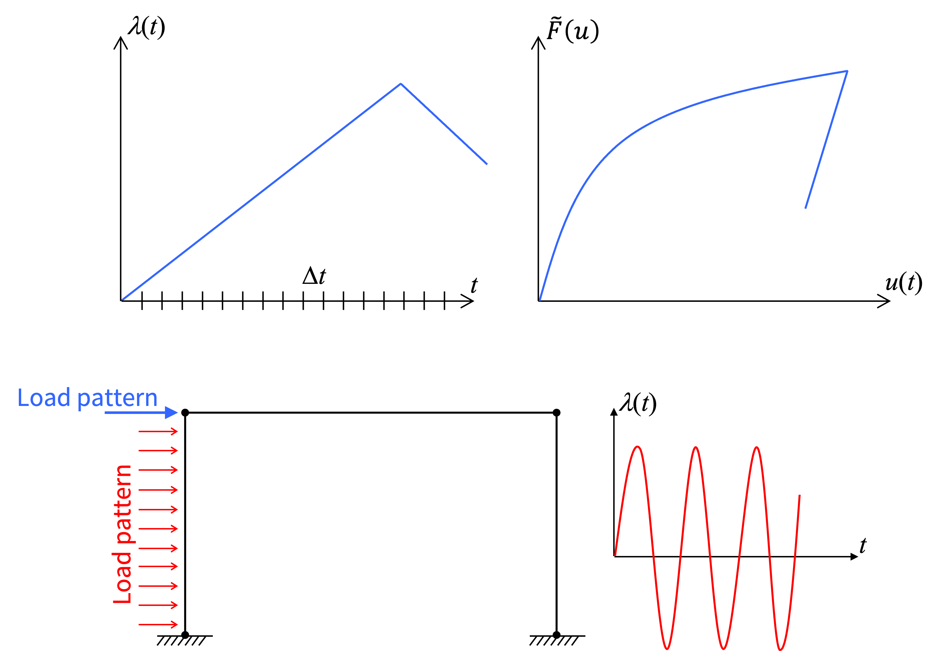
Equation 8.1 is solved step by step. The consecutive steps are called increments and it is helpful to think of them laid out along a pseudo time axis. In that way, one or more time series, like those in Figure 8.1, give the value of one or more load factors, \(\lambda(t)\), at each time increment. Although dynamic inertia forces are not present, using time in this manner facilitates a variety of loading and unloading scenarios, which hysteretic material models are made for. The load vector is therefore written
\[ \mathbf{F}(t) = \sum\limits_{k=1}^{K} \lambda_k(t) \cdot \mathbf{F}^{\mathrm{pattern}}_k \tag{8.2}\]
where \(\lambda_k\) is the load factor for “load pattern” number \(k\), with \(\mathbf{F}^{\mathrm{pattern}}_k\) representing the load vector that does not change along the pseudo time axis. Figure 8.1 illustrates the concepts of time series, load factors, and time-invariant load patterns.
8.1 Newton-Raphson Method
In the following, we seek the solution to Equation 8.1 at increment \(t_{n+1}\) assuming that the solution at time step \(t_{n}\) is already found. The interval between those pseudo times, i.e., \(\Delta t = t_{n+1} - t_n\), is in this book taken to be constant throughout the analysis. In fact, the code developed below takes \(\Delta t\) and number of time increments as input. In that way, the algorithm “pushes the analysis forward” by setting \(t_{n+1} = t_n + \Delta t\) at the start of each analysis increment. To that end, the rewritten version of Equation 8.1 is
\[ \tilde{\mathbf{F}}(\mathbf{u}_{n+1}) = \mathbf{F}(t_{n+1}) \tag{8.3}\]
where \(\mathbf{u}_{n+1}\) is the unknown displacement vector at time \(t_{n+1}\). Equation 8.3 is nonlinear in \(\mathbf{u}_{n+1}\) and therefore requires an iterative solution procedure. To derive the Newton-Raphson algorithm for this problem, Equation 8.3 is first written on residual form:
\[ \mathbf{R}(\mathbf{u}_{n+1}) = \tilde{\mathbf{F}}(\mathbf{u}_{n+1}) - \mathbf{F}(t_{n+1}) = \mathbf{0} \tag{8.4}\]
Next, the residual is expressed by a first-order Taylor approximation. The displacement about which the approximation is developed is given the index \(i\) and the displacement at which we seek the first-order approximation is at index \(i+1\). In summary, \(i\) is the index of the iterations towards solving Equation 8.4 and \(n\) is the index of the load increments at which that equation is solved. A precise but cumbersome notation for the Taylor linearization of the residual is
\[ \mathbf{R}(\mathbf{u}_{n+1,i+1}) \approx \mathbf{R}(\mathbf{u}_{n+1,i}) + \frac{\partial \mathbf{R}(\mathbf{u}_{n+1,i})}{\partial \mathbf{u}} \left(\mathbf{u}_{n+1,i+1}-\mathbf{u}_{n+1,i} \right) \tag{8.5}\]
A version that is more readable and also more helpful for subsequent implementations acknowledges the following:
- All iterations take place at increment \(n+1\), so that subscript can be omitted
- The derivative of the residual with respect to the displacement vector is effectively the derivative of the internal forces with respect to the displacement, which is the tangent stiffness, denoted by \(\mathbf{K}\)
- The parenthesis in Equation 8.5 is better written \(\Delta \mathbf{u}\) because hysteretic material models require incremental displacements, not total displacements
Those items give the following revised version of Equation 8.5:
\[ \mathbf{R}(\mathbf{u}_{i+1}) \approx \mathbf{R}(\mathbf{u}_i) + \mathbf{K}_i \Delta \mathbf{u}_i \tag{8.6}\]
Setting that linearized residual equal to zero per Equation 8.4 and rearrranging gives the linear system of equations solved repeatedly in the iterations of the algorithm conceived by Isaac Newton and cleaned up and made implementable by Joseph Raphson in the late 1600s:
\[ \mathbf{K}_i \Delta \mathbf{u}_i = -\mathbf{R}(\mathbf{u}_i) \tag{8.7}\]
It is stressed that \(\Delta \mathbf{u}_i\) means \(\mathbf{u}_{i+1} - \mathbf{u}_i\) at load increment \(n+1\). Starting at \(\mathbf{u}_1=\mathbf{0}\), or the displacements at the previously converged load increment if that is available, the Newton-Raphson iterations repeatedly solves Equation 8.7 for \(\Delta \mathbf{u}_i\). Each time, it sends three displacement vectors to the elements, cross-sections, and materials of the structure to assemble \(\tilde{\mathrm{F}}\) and \(\mathbf{K}\) to evaluate the residual and prepare for a new iteration. Those three displacements are:
- The solution to Equation 8.7, i.e., \(\Delta \mathbf{u}_i\), which is rarely but possibly used by some specialized elements. We call this the iteration displacement.
- The cumulative displacement within a load increment, \(\Delta \mathbf{u}_{\mathrm{increment}}=\mathbf{u}_1+\mathbf{u}_2+\mathbf{u}_3+\cdots\) employed by all hysteretic material models. We call this the incremental displacement.
- The total displacement accumulated over both iterations and increments, i.e., \(\mathbf{u}_n + \Delta \mathbf{u}_{\mathrm{increment}}\), used by linear elastic elements whose internal forces are not path-dependent. We call this the total displacement.
The code presented later in this chapter sends those three displacements to the elements, cross-sections, and materials of the structure at every Newton-Raphson iteration. In addition to the internal forces \(\tilde{\mathrm{F}}\), in return comes the tangent stiffness matrix for solving Equation 8.7. However, the Newton-Raphson algorithm may not use the updated stiffness. The analyst is usually given two options:
- Update the stiffess at every iteration at each load increment; this is called regular Newton-Raphson
- Do not update the stiffness but use the stiffness from the first iteration of the first load increment; this is called modified Newton-Raphson
Regular Newton-Raphson has quadratic convergence and thus converges quicker than modified Newton-Raphson, which exhibits linear convergence. However, for complex material models and structures, modified Newton-Raphson can be a more robust option. That is because it is usually less prone to non-convergence due to rapidly changing local stiffness values or bugs in the implementation of stiffness expressions in the elements, cross-sections, and materials. However, response sensitivity analysis is an important ingredient in this book. Having the updated stiffness after convergence, before the sensitivity calculations, is vital for accurate sensitivity results. After the response sensitivities are derived below, a summary of the complete sensitivity-enabled Newton-Raphson algorithm is presented.
8.1.1 First Differentiation
To derive response sensitivities by the DDM it is important to recognize that the generic variable \(x\) that we seek response sensitivities with respect to affects the internal forces in the left-hand side of Equation 8.1 in two ways. It always affects the response \(\mathbf{u}\), regardless of whether \(x\) is a load variable or a material property. That means \(\tilde{\mathbf{F}}\) is always affected by \(x\) in an implicit manner via \(\mathbf{u}\). However, \(\tilde{\mathbf{F}}\) also has an explicit dependence on \(x\) if that variable directly enters the algorithm that evaluates \(\tilde{\mathbf{F}}\). Examples of that are provided in this chapter. The implicit and explicit dependence are expressed in this revised version of Equation 8.1:
\[ \tilde{\mathbf{F}}(\mathbf{u}_{n+1}(x), x) = \lambda(t_{n+1}) \cdot \mathbf{F}^{\mathrm{pattern}}(x) \tag{8.8}\]
Only one load pattern and thus one load factor is considered, for brevity. The implicit and explicit dependence in the left-hand side require the use of the chain rule of differentiation to derive response sensitivities. First, as a basic illustration, consider a mathematical function formulated in terms of \(x\), \(y\), and \(z\) in the following manner: \(f(y(x), z(x))\). The chain rule says that the derivative of \(f\) with respect to \(x\) is \(\frac{\partial f}{\partial x}=\frac{\partial f}{\partial y}\frac{\partial y}{\partial x}+\frac{\partial f}{\partial z}\frac{\partial z}{\partial x}\). Embedded in this rule is that \(z\) is fixed in the differentiation in the first term and \(y\) is fixed in the differentiation in the second term. That is why, if the function is formulated as \(f(y(x), x)\) the derivative is \(\frac{\partial f}{\partial y}\frac{\partial y}{\partial x}+\frac{\partial f}{\partial x}\) with the understanding that the differentiation in the last term is carried out for fixed \(y\). This is why the differentiation of Equation 8.8 gives
\[ \frac{\partial \tilde{\mathbf{F}}(\mathbf{u}_{n+1})}{\partial \mathbf{u}} \frac{\partial \mathbf{u}_{n+1}}{\partial x} + \left. \frac{\partial \tilde{\mathbf{F}}(\mathbf{u}_{n+1})}{\partial x} \right|_{\mathbf{u}_{n+1} \: \mathrm{fixed}} = \lambda(t_{n+1}) \cdot \frac{\partial \mathbf{F}^{\mathrm{pattern}}}{\partial x} \tag{8.9}\]
where the stiffness matrix at the converged equilibrium state at load increment \(n+1\) is the first factor in the first term: \(\frac{\partial \tilde{\mathbf{F}}(\mathbf{u}_{n+1})}{\partial \mathbf{u}} \equiv \mathbf{K}(\mathbf{u}_{n+1})\). Rearranging Equation 8.9 gives a linear system of equations with the same coefficient matrix as the linear system of equations in Equation 8.7:
\[ \mathbf{K}(\mathbf{u}_{n+1}) \frac{\partial \mathbf{u}_{n+1}}{\partial x} = \lambda(t_{n+1}) \cdot \frac{\partial \mathbf{F}^{\mathrm{pattern}}}{\partial x} - \left. \frac{\partial \tilde{\mathbf{F}}(\mathbf{u}_{n+1})}{\partial x} \right|_{\mathbf{u}_{n+1} \: \mathrm{fixed}} \tag{8.10}\]
The fact that response sensitivities are solved from a single linear system of equations after convergence of the Newton-Raphson algorithm is a general characteristic of the DDM. However, it is reiterated that the matrix \(\mathbf{K}(\mathbf{u}_{n+1})\) in Equation 8.10 must be the updated tangent stiffness matrix calculated at the converged equilibrium state.
Key to understanding the DDM for nonlinear problems is that “\(\mathbf{u}_{n+1} \: \mathrm{fixed}\)” in Equation 8.9 means fixed only at the current time step. It does not mean “\(\mathbf{u}_{n} \: \mathrm{fixed}\).” In fact, the differentiation must be carried out with displacements at all previous load increments free. Adopting that understanding, explained by Zhang and Der Kiureghian (1993), conditional derivatives must first be calculated and Equation 8.9 solved for \(\frac{\partial \mathbf{u}_{n+1}}{\partial x}\), followed by the calculation of unconditional derivatives of \(\tilde{\mathbf{F}}\), using exactly that sensitivity \(\frac{\partial \mathbf{u}_{n+1}}{\partial x}\), in preparation for the next time step. This is shown in the sensitivity-enabled Newton-Raphson algorithm presented shortly and implemented in the code presented later in the chapter.
8.1.2 Second Differentiation
Exact second-order response sensitivities are obtained by differentiating the governing equations in Equation 8.8 twice. The first differentiation is already available in Equation 8.9. The second differentiation must account for these facts:
The variable that the first differentiation was carried out with respect to, now lablled \(x_i\) may be different from the variable in the second differentiation, here labelled \(x_j\)
Because the stiffness matrix \(\mathbf{K}(\mathbf{u}_{n+1})\) that appears in Equation 8.9 depends on the displacement, the same implicit-explicit differentiation behind the two terms in the left-hand side of that equation appear also in the differentiation of \(\mathbf{K}(\mathbf{u}_{n+1})\)
Although the conditional derivative \(\left. \frac{\partial \tilde{\mathbf{F}}(\mathbf{u}_{n+1})}{\partial x} \right|_{\mathbf{u}_{n+1} \: \mathrm{fixed}}\) that appears in Equation 8.9 is carried out for fixed current displacements, the resulting derivative depends on the displacement. Thus, again, the implicit-explicit differentiation gives two terms because the differentiation must be carried out in the manner described in the previous subsection.
In conclusion, the second differentiation yields five terms from the two terms in the left-hand side of Equation 8.9, one of those terms being associated with the product rule of differentiation:
\[ \begin{aligned} &\frac{\partial \mathbf{K}(\mathbf{u}_{n+1})}{\partial \mathbf{u}} \frac{\partial \mathbf{u}_{n+1}}{\partial x_j} \frac{\partial \mathbf{u}_{n+1}}{\partial x_i} \\ &+ \left. \frac{\partial \mathbf{K}(\mathbf{u}_{n+1})}{\partial x_j} \right|_{\mathbf{u}_{n+1} \: \mathrm{fixed}} \frac{\partial \mathbf{u}_{n+1}}{\partial x_i} \\ &+ \mathbf{K}(\mathbf{u}_{n+1}) \frac{\partial^2 \mathbf{u}_{n+1}}{\partial x_i \partial x_j} \\ &+ \left. \frac{\partial \mathbf{K}(\mathbf{u}_{n+1})}{\partial x_i} \right|_{\mathbf{u}_{n+1} \: \mathrm{fixed}} \frac{\partial \mathbf{u}_{n+1}}{\partial x_j} \\ &+ \left. \frac{\partial^2 \tilde{\mathbf{F}}(\mathbf{u}_{n+1})}{\partial x_i \partial x_j} \right|_{\mathbf{u}_{n+1} \: \mathrm{fixed}} = \lambda(t_{n+1}) \cdot \frac{\partial^2 \mathbf{F}^{\mathrm{pattern}}}{\partial x_i \partial x_j} \end{aligned} \tag{8.11}\]
Notice that the second-last term in the left-hand side is obtained by flipping the order of differentiation with respect to \(x_i\) and \(\mathbf{u}\), which is why the stiffness, i.e., \(\frac{\partial \tilde{\mathbf{F}}}{\partial \mathbf{u}}\), appears in that term. Rearranging Equation 8.11, keping only the third term on the left-hand side, again reveals a linear system of equations for the second-order response sensitivities, a staple of the DDM:
\[ \mathbf{K}(\mathbf{u}_{n+1}) \frac{\partial^2 \mathbf{u}_{n+1}}{\partial x_i \partial x_j} = (\cdots) \tag{8.12}\]
Same as with Equation 8.11 it is stressed that \(\mathbf{K}(\mathbf{u}_{n+1})\) must be the tangent stiffness consistent with the converged state at the last Newton-Raphson iteration of the load increment \(n+1\). In contrast to the governing equations presented in Chapter 1 for first- and second-order sensitivities in linear elastic analysis, the adjoint method is not applicable in nonlinear analysis. That is because the full vectors \(\mathbf{u}_{n+1}\), \(\frac{\partial \mathbf{u}_{n+1}}{\partial x}\), and \(\frac{\partial^2 \mathbf{u}_{n+1}}{\partial x_i \partial x_j}\) are required to calculate and save the unconditional derivatives for subsequent increments, as described in the last paragraph of Section 8.1.1. In fact, Equation 8.11 for second-order sensitivities requires the same two steps as the first-order sensitivity calculations described earlier: First conditional derivatives are calculated, then unconditional derivatives are calculated and stored in the hysteretic material models once sensitivities are solved for. That point, which echoes Bebamzadeh and Haukaas (2008), is embedded in the sensitivity-enhanced Newton-Raphson algorithm described next.
8.1.3 Amended Newton-Raphson
The phrase state determination was briefly mentioned in Chapter 3. Now its necessity becomes clear. In nonlinear analysis, the state determination in the structure, or an element, or a cross-section, or a material model carries a specific job description. Take the trial displacements produced by Equation 8.7 and calculate two things:
The resisting forces \(\tilde{\mathbf{F}}(\mathbf{u}_{n+1})\) required to check if the residual in Equation 8.6 is zero
The tangent stiffness \(\mathbf{K}(\mathbf{u}_{n+1})\) required to solve Equation 8.7 yet again, until convergence, and thereafter to calculate response sensitivities via Equation 8.9 and Equation 8.11
Hysteretic material models contain history variables that are needed to calculate the stress for a new strain increment. Once the Newton-Raphson algorithm converges at a load increment, the trial values of the history variables that were temporarily calculated during the Newton-Raphson iterations are stored for use in the next increment. In other words, the Newton-Raphson algorithm must issue a call to commit the history variables once convergence is achieved. This is why a commit() function always accompany a stateDetermination() function.
That pair of functions, seen in every element, cross-section, and material instance, is complemented with function pairs for sensitivity analysis. The previously described fact that the conditional derivatives in Equation 8.9 and Equation 8.11 are only conditional on fixed current displacements, not previously committed displacements, gives the following sensitivity-enhanced Newton-Raphson algorithm:
- Issue
stateDetermination()call to establish the initial stiffness matrix, \(\mathbf{K}\) - Initialize to zero the internal force vector, \(\tilde{\mathbf{F}}\)
- Loop over load increments (\(n\) counter):
- Evaluate the right-hand side of Equation 8.3 to establish the load vector, \(\mathbf{F}\)
- Loop over Newton-Raphson iterations (\(i\) counter):
- Use Equation 8.4 to evaluate the residual, \(\mathbf{R}\)
- Check convergence, e.g., whether \(\lVert \mathbf{R} \rVert < \mathrm{tolerance}\)
- Solve the linear system of equations in Equation 8.7 for \(\Delta \mathbf{u}_i\)
- With new trial displacements, issue
stateDetermination()call to get internal forces, \(\tilde{\mathbf{F}}\), and tangent stiffness, \(\mathbf{K}\) - Upon convergence:
- Do NOT commit trial history variables in the hysteretic materials yet
- Make sure that the stiffness matrix is up-to-date for the subsequent sensitivity calculations
- Call
stateDerivative()to calculate \(\left. \frac{\partial \tilde{\mathbf{F}}}{\partial x} \right|_{\mathbf{u} \: \mathrm{fixed}}\) for Equation 8.9 - Solve Equation 8.10 for \(\frac{\partial \mathbf{u}}{\partial x}\)
- Call
commitSensitivity()with the first-order sensitivities from the previous item so that hysteretic material models can store unconditional derivatives of the history variables - Call
stateSecondDerivative()to calculate \(\left. \frac{\partial \mathbf{K}}{\partial x_i} \right|_{\mathbf{u} \: \mathrm{fixed}}\) and \(\left. \frac{\partial^2 \tilde{\mathbf{F}}}{\partial x_i \partial x_j} \right|_{\mathbf{u} \: \mathrm{fixed}}\) for Equation 8.11 - Solve Equation 8.12 for \(\frac{\partial^2 \mathbf{u}}{\partial x_i \partial x_j}\)
- Call
commitSecondSensitivity()with the second-order sensitivities from the previous item so that hysteretic material models can store unconditional second-order derivatives of the history variables - Issue
commit()call to store trial history variables in hysteretic material objects, for use in the next increment; notice that this call must be made after the sensitivity calculations
That algorithm is implemented below, after first developing a nonlinear material and nonlinear element to test it on. In doing so, notice that the unconditional derivatives stored by the calls to commitSensitivity() and commitSecondSensitivity() are vectors and matrices, respectively, with dimensions equal to the number of variables in \(\mathbf{x}\) for which response sensitivities are sought.
8.2 Bilinear Material
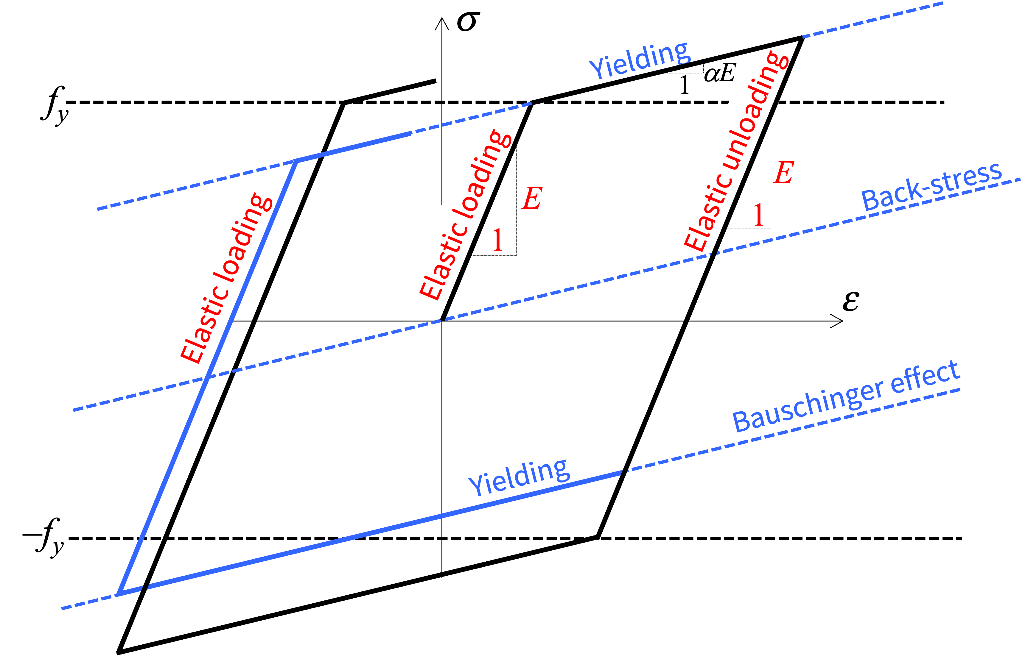
The uniaxial material model visualized in Figure 8.2 is relatively simple but yet popular. Highlighted in blue, it accommodates the Bauschinger effect, i.e., yielding before the yield stress, \(f_y\), after prior yielding in the other direction. This is called kinematic hardening, manifesting as a uniform shift in the elastic region quantified by the back stress. Also notice in Figure 8.2 that the stiffness after yielding is \(\alpha \cdot E\), where \(E\) is the initial stiffness, and that unloading is elastic, following that initial stiffness.
Uniaxial material models like the one in Figure 8.2 is useful in several applications. One example presented in this chapter is a nonlinear truss element. However, the range of applications for a uniaxial material model go beyond truss elements. In the next chapter, a distributed plasticity element with a fibre-discretized cross-section is presented, with a uniaxial material in every fibre.
This model accommodates various loading and unloading scenarios when receiving a strain increment. Specifically, it is the incremental strain from the Newton-Raphson algorithm that the material model employs for this purpose. Following the definitions made earlier in this chapter, that is the second of three strains given to the material, which is why deps[1] appears in the code shown below. Notice how the if statements in the following state determination deal will all possible loading and unloading scenarios:
def stateDetermination(self, eps):

    # Incremental strain
    deps = eps[1]

    # Check for unloading
    unloading = False
    if (self.committedYielding == True and (self.committedStress - self.committedBackStress) * deps < 0):
        unloading = True

    # Check if the last state was elastic or if the strain increment implies unloading from yielding
    if self.committedYielding is False or unloading:

        # Strain increment that would cause yielding
        depsToYield = (np.sign(deps) * self.fy + self.committedBackStress - self.committedStress) / self.E

        # Keep elastic state handy, in case that becomes the conclusion
        self.trialStress = self.committedStress + self.E * deps
        Et = self.E
        self.trialYielding = False

        # Check if the strain increment causes yielding from an elastic state (initiation of unloading is elastic)
        if abs(deps) > abs(depsToYield) and not unloading:
            self.trialStress = self.trialStress + (self.alpha * self.E - self.E) * (deps - depsToYield)
            self.trialBackStress = self.committedBackStress + self.alpha * self.E * (deps - depsToYield)
            Et = self.alpha * self.E
            self.trialYielding = True

    else:

        # Continue plastic loading
        self.trialStress = self.committedStress + self.alpha * self.E * deps
        self.trialBackStress = self.committedBackStress + self.alpha * self.E * deps
        Et = self.alpha * self.E
        self.trialYielding = True

    return self.trialStress, Et
In the end, we observe that the stress and tangent stiffness are returned for step 3-II-D of the Newton-Raphson algorithm in Section 8.1.3. Also, in the state determination above we observe a number self.trial data members. They are initialized in the constructor, and change value for every iteration of the Newton-Raphson algorithm. Once that algorithm converges, but after the sensitivity calculations, it issues the commit() call that prompts storage of trial values as self.committed counterparts serving as the starting point for the next load increment.
The complete code for the bilinear material model, with functions for first- and second-order sensitivity analysis, is too large to present in this chapter. Instead, that code is made available in Appendix A and imported here:
from AppendixAcode import *Including the state determination in Listing 8.1, the following member functions of the bilinear material class, meeting the requirements of the Newton-Rapshon algorithm in Section 8.1.3, are included in the appendix:
def __init__()(Constructor)def stateDetermination()def stateDerivative()def stateSecondDerivative()def commit()def commitSensitivity()def commitSecondSensitivity()
8.3 Nonlinear Truss Element
Earlier in this book, Element 5 was introduced as the linear elastic frame element. Conversely, Element 2 is a nonlinear truss element, meaning that it takes a uniaxial material model as input to represent its axial force-displacement relationship. In addition, it receives the intial axial force, \(N_0\), which is a placeholder for now, and the cross-section area, \(A\):
class element2():
    def __init__(self, N0, section, material, elno):
        self.no = elno
        self.N0 = N0
        self.A = float(section[1])
        self.mat = bilinearMaterial(material)
The element also has a function to initialize oft-used quantities, and ideally some error checking omitted here for brevity. For Element 2, it is the direction cosines, element length, and transformation from Basic to Global that are created at the initialization of the element:
class element2(element2):
    def initialize(self, xyz):
        dx = xyz[1,:] - xyz[0,:]
        self.L = np.sqrt(dx.dot(dx))
        dx = dx / self.L
        self.Tbg = np.array([-dx[0], -dx[1], dx[0], dx[1]])
That transformation “matrix” is a vector because of the single Basic axial DOF. It essentially picks up the first row in Equation 3.3 from Chapter 3:
\[ \mathbf{T} = \{ -\mathrm{cos}(\theta) \; -\mathrm{sin}(\theta) \; \mathrm{cos}(\theta) \; \mathrm{sin}(\theta)\} \tag{8.13}\]
8.3.1 State Determination
No distributed element load is implemented for the truss element. Hence, the Both point made for the force vector in Chapter 3 is mute here. It is only the displacement-resisting force vector,
\[ F_B = \sigma(\varepsilon) \cdot A \tag{8.14}\]
and associated stiffness,
\[ K_B = \frac{\partial F_B}{\partial u_B} = \frac{\partial F_B}{\partial \varepsilon} \frac{\partial \varepsilon}{\partial u_B} = \left(A \cdot \frac{\partial \sigma}{\partial \varepsilon}\right) \frac{1}{L} = \frac{E(\varepsilon)\cdot A}{L} \tag{8.15}\]
that are returned from the state determination in this element, with \(\sigma\) and \(E\) provided by its material object:
class element2(element2):
    def stateDetermination(self, xyz, ug, theLambda):
        ub = self.Tbg.dot(ug)
        epsilon = ub/self.L
        sigma, E = self.mat.stateDetermination(epsilon)
        Kb = E * self.A / self.L
        Fb = sigma * self.A + self.N0
        self.FbTrial = Fb
        Fg = np.multiply(Fb, self.Tbg)
        Kg = np.multiply(Kb, np.outer(self.Tbg, self.Tbg))
        return Fg, Kg
In Listing 8.4, notice that all three displacement components from the Newton-Raphson algorithm, i.e., total displacement, incremental displacement, and iteration displacement are passed on to the material as three strains contained in epsilon.
8.3.2 First-order Sensitivities
The right-hand side of Equation 8.10 requires the derivative of the vector of external loads, as well as the derivative of the internal resisting forces for fixed currente displacements. However, in the absence of distributed element loads in this element, only the latter is relevant. Differentiation of Equation 8.14 yields \[ \frac{\partial F_B}{\partial x} = \frac{\partial \sigma}{\partial x} \cdot A + \sigma \cdot \frac{\partial A}{\partial x} \tag{8.16}\]
As mentioned after Listing 3.3, the derivative of the stiffness is not required by the first-order sensitivity algorithm that calls the element. However, it is needed in second-order sensitivity calculations. Differentiation of Equation 8.15 gives
\[ \frac{\partial K_B}{\partial x} = \frac{\partial E}{\partial x}\cdot \frac{A}{L} + \frac{\partial A}{\partial x}\cdot \frac{E}{L} \tag{8.17}\]
Those derivatives are implemented in this function:
class element2(element2):
    def stateDerivative(self, xyz, ug, theLambda, ddmParameter, ddmIndex, ddmIsHere, dKflag='none'):
        ub = self.Tbg.dot(ug)
        epsilon = ub/self.L
        sigma, E = self.mat.stateDetermination(epsilon)
        dsigma, dE, dEdeps = self.mat.stateDerivative(epsilon, ddmParameter, ddmIndex, ddmIsHere, dKflag)
        dArea = 0.0
        if ddmParameter=='A' and ddmIsHere:
            dArea = 1.0
        dKb = dE * self.A / self.L + E * dArea / self.L
        dFb = dsigma * self.A + sigma * dArea
        dFg = self.Tbg.dot(dFb)
        dKg = np.outer(self.Tbg.dot(dKb), self.Tbg)
        if dKflag != 'none':
            A, B, C = np.ix_(self.Tbg, self.Tbg, self.Tbg)
            dKgdug = np.multiply(dEdeps * self.A / self.L**2, A * B * C)
        else:
            dKgdug = 0
        return dFg, dKg, dKgdug
The returned quantity dKgdug, also mentioned below Listing 3.3 for Element 5, will be explained in Chapter 12.
8.3.3 Second-order Sensitivities
In the absence of distributed element loads, and disregarding quantities already available, Equation 8.11 requires the element to provide the second-order derivative of the internal forces \(\tilde{\mathbf{F}}\). The second differentiation of Equation 8.16 yields
\[ \frac{\partial^2 F_B}{\partial x_i \partial x_j} = \frac{\partial^2 \sigma}{\partial x_i \partial x_j} \cdot A + \frac{\partial \sigma}{\partial x_i} \cdot \frac{\partial A}{\partial x_j} + \frac{\partial \sigma}{\partial x_j} \cdot \frac{\partial A}{\partial x_i} \tag{8.18}\]
That formula is seen in the third-to-last line in the following implementation:
class element2(element2):
    def stateSecondDerivative(self, xyz, ug, theLambda, secondOrderIndex, ddmParameter1, ddmIndex1, ddmIsHere1, ddmParameter2, ddmIndex2, ddmIsHere2):
        ub = self.Tbg.dot(ug)
        epsilon = ub/self.L
        dsigma1, dE1, void = self.mat.stateDerivative(epsilon, ddmParameter1, ddmIndex1, ddmIsHere1)
        dsigma2, dE2, void = self.mat.stateDerivative(epsilon, ddmParameter2, ddmIndex2, ddmIsHere2)
        ddsigma, ddE = self.mat.stateSecondDerivative(epsilon, secondOrderIndex, ddmParameter1, ddmIndex1, ddmIsHere1, ddmParameter2, ddmIndex2, ddmIsHere2)
        dArea1 = 0.0
        if ddmParameter1=='A' and ddmIsHere1:
            dArea1 = 1.0
        dArea2 = 0.0
        if ddmParameter2=='A' and ddmIsHere2:
            dArea2 = 1.0
        ddFb = ddsigma * self.A + dsigma1 * dArea2 + dsigma2 * dArea1
        ddFg = self.Tbg.dot(ddFb)
        return ddFg
8.3.4 Commit
The commit() call after convergence of the Newton-Raphson algorithm at a load increment is related to history variables. These variables reside in hysteretic material models, which is why the truss element simply conveys the call to its material object:
class element2(element2):
    def commit(self, xyz, u):
        self.mat.commit()
The need for derivatives that are conditional only on fixed current displacements is explained in Section 8.1.1. That issue prompts two calls from the orchestrating algorithm to calculate first-order sensitivities at the end of every load increment. The first call is addressed above; the second call is made after calculation of the sensitivities, now storing unconditional derivatives of the history variables:
class element2(element2):
    def commitSensitivity(self, xyz, ug, dug, ddmParameter, ddmIndex, ddmIsHere):
        ub = self.Tbg.dot(ug)
        epsilon = ub/self.L
        dub = self.Tbg.dot(dug)
        ddmepsilon = dub/self.L
        self.mat.commitSensitivity(epsilon, ddmepsilon, ddmParameter, ddmIndex, ddmIsHere)
Similarly, the second call to store unconditional second-order derivatives of history variables is conveyed to the material object with the following member function of the element class:
class element2(element2):
    def commitSecondSensitivity(self, xyz, ug, dug1, dug2, ddug, secondOrderIndex, ddmParameter1, ddmIndex1, ddmIsHere1, ddmParameter2, ddmIndex2, ddmIsHere2):
        ub = self.Tbg.dot(ug)
        epsilon = ub/self.L
        dub1 = self.Tbg.dot(dug1)
        depsilon1 = dub1/self.L
        dub2 = self.Tbg.dot(dug2)
        depsilon2 = dub2/self.L
        ddub = self.Tbg.dot(ddug)
        ddepsilon = ddub/self.L
        self.mat.commitSecondSensitivity(epsilon, depsilon1, depsilon2, ddepsilon, secondOrderIndex, ddmParameter1, ddmIndex1, ddmIsHere1, ddmParameter2, ddmIndex2, ddmIsHere2)
8.3.5 Add Element to Model
The nonlinear truss element whose member functions are developed and implemented above is now added to the structural model. As a result, elements of type Element 2 and Element 5 can now be created:
class model(model):
    def createElements(self):
        nelem = len(self.ELEMENTS)
        ellist = []
        for i in range(nelem):
            eltyp = self.ELEMENTS[i][0]
            if eltyp == 5:
                E = self.ELEMENTS[i][1]
                A = self.ELEMENTS[i][2]
                I = self.ELEMENTS[i][3]
                q = self.ELEMENTS[i][4]
                el = element5(E, A, I, q, i+1)
            elif eltyp == 2:
                N0 = self.ELEMENTS[i][1]
                el = element2(N0, self.SECTIONS[i], self.MATERIALS[i], i+1)
            ellist.append(el)
        return ellist
8.4 Analysis Algorithm
The time series concept is explained at the start of this chapter. A simple implementation is provided here, facilitating loading, unloading, and reloading. The load factor, \(\lambda\), first increases linearly with time, peaking at \(\lambda(t=1)=1\). Then the load factor starts a linear decline, passing \(\lambda=0\) at \(t=2\), peaking on the negative side at \(\lambda(t=3)=-1\). Thereafter it increases linearly with no end:
def timeSeries(t):
    if t<1.0:
        theLambda = t
    elif t<3.0:
        theLambda = 1.0-(t-1.0)
    else:
        theLambda = -1.0+(t-3.0)
    return theLambda
Here is that time series visualized:
t = np.linspace(0, 4.5, 100)
lamda = []
for i in range(len(t)):
    lamda.append(timeSeries(t[i]))
plt.figure()
plt.plot(t, lamda, 'k-')
plt.xlabel("Pseudo time, $t$")
plt.ylabel("Load factor, $\\lambda$")
plt.grid(True)
plt.show()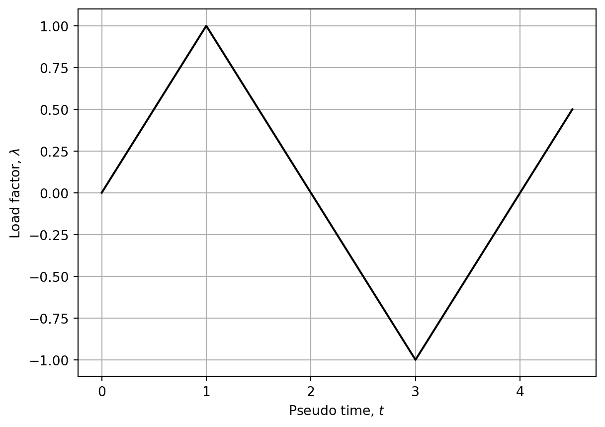
A single function is provided below to calculate the response alongside first- and second-order response sensitivities. Comment lines identify the start of increments, iterations, as well as the start of first- and second-order sensitivity calculations. The following comments are added:
- As usual, error checks are omitted for brevity. It is prudent to check that the given variable name actually exists, etc.
- Notice how all elements must be called in the sensitivity analysis, regardless of whether the variable resides in the element. That is because the element might still supply non-zero contributions to the sensitivity calculations. This is a unique feature of structural analysis with hysteretic material models. It turns out the exception to this rule is statically determinate structures; there, the element provides non-zero sensitivity contributions only if the variable resides in it.
- The storage of unconditional derivatives for the next load increment is another feature of sensitivity analysis with hysteretic material models. The unconditional derivative of each history variables with respect to each variable is stored in the call to
commitSensitivity. Similarly, for each history variable, a matrix of unconditional cross-derivatives is stored in the call tocommitSecondSensitivity. - The algorithm presented below does not accommodate modified Newton-Raphson; here, the tangent stiffness is updated at every iteration of every increment.
- The
tildelabel is applied to certain force vectors, as seen below. In analyses in subsequent chapters, some of those vectors will include contributions from distributed element loads, as described earlier. However, thetildelabel is kept here, matching the notation established in Equation 8.1.
from scipy.linalg import lu_factor, lu_solve
def nonlinearStaticAnalysis(model, nsteps, dt, trackNode, trackDOF, DDMparameters=[], ddmRequest=0):
    maxiter = 100
    tol = 1e-5
    ndof, ntot, Fref, M, elemlist = model.getData()
    free = range(ndof)
    nelem = len(elemlist)
    Fa_tilde = np.zeros(ntot)
    Ka = np.zeros((ntot, ntot))
    ua = np.zeros((ntot, 3))
    if len(DDMparameters) > 0 and ddmRequest > 0:
        ddmua = np.zeros(ntot)
    if isinstance(trackNode, list):
        trackNode = trackNode[0]
    if isinstance(trackDOF, list):
        trackDOF = trackDOF[0]
    dof = model.DOF[trackNode - 1, trackDOF - 1]
    for i in range(nelem):
        id, xyz, ug = model.localize(i, ua[:,0])
        elemlist[i].initialize(xyz)
    uTrack = []
    trackTime = []
    loadFactor = []
    time = 0.0
    dudx = np.zeros((len(DDMparameters), nsteps))
    dudx2 = np.zeros((len(DDMparameters), len(DDMparameters), nsteps))

    # Increments
    for increment in range(nsteps):
        time += dt
        theLambda = timeSeries(time)
        Fa = theLambda * Fref

        # Iterations
        for i in range(maxiter):
            Fa_tilde[:] = 0.0
            Ka[:] = 0.0
            for j in range(nelem):
                id, xyz, ug = model.localize(j, ua)
                element = elemlist[j]
                Fg_tilde, Kg = element.stateDetermination(xyz, ug, theLambda)
                Fa_tilde[id] = Fa_tilde[id] + Fg_tilde
                Ka[np.ix_(id, id)] = Ka[np.ix_(id, id)] + Kg
            Rf = Fa_tilde[free] - Fa[free]
            residualNorm = np.linalg.norm(Rf)
            if residualNorm < tol:
                break
            Kf = Ka[np.ix_(free, free)]
            ua[free, 2] = np.linalg.solve(Kf, -Rf)
            ua[:, 0] = ua[:, 0] + ua[:, 2]
            ua[:, 1] = ua[:, 1] + ua[:, 2]
        if residualNorm > tol:
            print(f"\nNo convergence with residual {residualNorm} > {tol} in {maxiter} iterations at increment {increment+1}")

        # Sensitivity analysis
        if len(DDMparameters) > 0 and ddmRequest > 0:
            Kf = Ka[np.ix_(free, free)]
            LU = lu_factor(Kf)
            dKfdxStorage = []
            dKfduStorage = []
            dufdxStorage = []

            # First-order sensitivities
            for ddmIndex in range(len(DDMparameters)):
                ddmRHSa = np.zeros(ntot)
                dKa = np.zeros((ntot, ntot))
                dKadua = np.zeros((ntot, ntot, ntot))
                if DDMparameters[ddmIndex][0] == 'Element':
                    ddmIsHere = np.full(nelem, False)
                    for eleNum in DDMparameters[ddmIndex][2]:
                        ddmIsHere[eleNum - 1] = True
                    for i in range(nelem):
                        id, xyz, ug = model.localize(i, ua)
                        element = elemlist[i]
                        dFg, dKg, dKgdug = element.stateDerivative(xyz, ug, theLambda, DDMparameters[ddmIndex][1], ddmIndex, ddmIsHere[i])
                        ddmRHSa[id] = ddmRHSa[id] - dFg
                        dKa[np.ix_(id, id)] = dKa[np.ix_(id, id)] + dKg
                        if not np.isscalar(dKgdug):
                            dKadua[np.ix_(id, id, id)] = dKadua[np.ix_(id, id, id)] + dKgdug
                elif DDMparameters[ddmIndex][0] == 'Nodal load':
                    loadIndex = model.DOF[DDMparameters[ddmIndex][1] - 1, DDMparameters[ddmIndex][2] - 1]
                    ddmRHSa[loadIndex] = theLambda * np.sign(Fa[loadIndex])
                    for i in range(nelem):
                        id, xyz, ug = model.localize(i, ua)
                        element = elemlist[i]
                        dFg, dKg, dKgdug = element.stateDerivative(xyz, ug, theLambda, DDMparameters[ddmIndex][1], ddmIndex, False)
                        ddmRHSa[id] = ddmRHSa[id] - dFg
                        dKa[np.ix_(id, id)] = dKa[np.ix_(id, id)] + dKg
                        if not np.isscalar(dKgdug):
                            dKadua[np.ix_(id, id, id)] = dKadua[np.ix_(id, id, id)] + dKgdug
                ddmRHSf = ddmRHSa[free]
                ddmDisplacementNew = lu_solve(LU, ddmRHSf)
                ddmua[free] = ddmDisplacementNew
                dudx[ddmIndex, increment] = ddmua[dof]
                if ddmRequest > 1:
                    dKfdxStorage.append(dKa[np.ix_(free, free)])
                    dKfduStorage.append(dKadua[np.ix_(free, free, free)])
                    dufdxStorage.append(ddmDisplacementNew[np.ix_(free)])

                # Commit unconditional first-order derivatives
                if DDMparameters[ddmIndex][0] == 'Element':
                    for i in range(nelem):
                        id, xyz, ug = model.localize(i, ua)
                        id, xyz, ddmug = model.localize(i, ddmua)
                        element = elemlist[i]
                        element.commitSensitivity(xyz, ug, ddmug, DDMparameters[ddmIndex][1], ddmIndex, ddmIsHere[i])
                elif DDMparameters[ddmIndex][0] == 'Nodal load':
                    for i in range(nelem):
                        id, xyz, ug = model.localize(i, ua)
                        id, xyz, ddmug = model.localize(i, ddmua)
                        element = elemlist[i]
                        element.commitSensitivity(xyz, ug, ddmug, DDMparameters[ddmIndex][1], ddmIndex, False)

            # Second-order sensitivities
            if ddmRequest > 1:
                secondOrderIndex = -1
                for ddmIndex2 in range(len(DDMparameters)):
                    for ddmIndex1 in range(ddmIndex2+1):
                        secondOrderRHSa = np.zeros(ntot)
                        secondOrderIndex += 1
                        if DDMparameters[ddmIndex1][0] == 'Element' and DDMparameters[ddmIndex2][0] == 'Element':
                            ddmIsHere1 = np.full(nelem, False)
                            for eleNum in DDMparameters[ddmIndex1][2]:
                                ddmIsHere1[eleNum - 1] = True
                            ddmIsHere2 = np.full(nelem, False)
                            for eleNum in DDMparameters[ddmIndex2][2]:
                                ddmIsHere2[eleNum - 1] = True
                            for i in range(nelem):
                                id, xyz, ug = model.localize(i, ua)
                                element = elemlist[i]
                                ddFg = element.stateSecondDerivative(xyz, ug, theLambda, secondOrderIndex, DDMparameters[ddmIndex1][1], ddmIndex1, ddmIsHere1[i], DDMparameters[ddmIndex2][1], ddmIndex2, ddmIsHere2[i])
                                secondOrderRHSa[id] = secondOrderRHSa[id] - ddFg
                        elif DDMparameters[ddmIndex][0] == 'Nodal load':
                            for i in range(nelem):
                                id, xyz, ug = model.localize(i, ua)
                                element = elemlist[i]
                                ddFg = element.stateSecondDerivative(xyz, ug, theLambda, secondOrderIndex, DDMparameters[ddmIndex1][1], ddmIndex1, False, DDMparameters[ddmIndex2][1], ddmIndex2, False)
                                secondOrderRHSa[id] = secondOrderRHSa[id] - ddFg
                        secondOrderRHSf = secondOrderRHSa[free] - dKfdxStorage[ddmIndex1].dot(dufdxStorage[ddmIndex2])
                        parenthesis = np.einsum('ijk,k->ij', dKfduStorage[ddmIndex2], dufdxStorage[ddmIndex2]) + dKfdxStorage[ddmIndex2]
                        secondOrderRHSf = secondOrderRHSf - parenthesis.dot(dufdxStorage[ddmIndex1])
                        secondOrderDisplacementSensitivity = lu_solve(LU, secondOrderRHSf)
                        dudx2[ddmIndex1, ddmIndex2, increment] = secondOrderDisplacementSensitivity[dof]
                        dudx2[ddmIndex2, ddmIndex1, increment] = secondOrderDisplacementSensitivity[dof]

                        # Commit unconditional second-order derivatives
                        for i in range(nelem):
                            id, xyz, ug = model.localize(i, ua)
                            ddmua[free] = dufdxStorage[ddmIndex1]
                            id, xyz, dug1 = model.localize(i, ddmua)
                            ddmua[free] = dufdxStorage[ddmIndex2]
                            id, xyz, dug2 = model.localize(i, ddmua)
                            ddmua[free] = secondOrderDisplacementSensitivity
                            id, xyz, ddug = model.localize(i, ddmua)
                            element = elemlist[i]
                            element.commitSecondSensitivity(xyz, ug, dug1, dug2, ddug, secondOrderIndex, DDMparameters[ddmIndex1][1], ddmIndex1, ddmIsHere1[i], DDMparameters[ddmIndex2][1], ddmIndex2, ddmIsHere2[i])

        # Regular Newton-Raphson commit call, AFTER sensitivity analysis
        for i in range(nelem):
            id, xyz, ug = model.localize(i, ua)
            element = elemlist[i]
            element.commit(xyz, ug)
        ua[:, 1] = 0.0
        uTrack.append(ua[dof, 0])
        trackTime.append(time)
        loadFactor.append(theLambda)

    return trackTime, loadFactor, uTrack, dudx, dudx2
The five returned quantities are:
- Array that contains the time axis, \(\mathbf{t}\)
- Value of the load factor, \(\lambda\), at every time increment
- Displacement response, \(u\), at every time increment
- Matrix of first-order response sensitivities, \(\frac{\partial u[i, n]}{\partial x_i}\), where \(i\) is the index of the variable and \(n\) is the index of the time increment, meaning we get sensitivities at \(\mathbf{t}[n]\)
- Tensor of second-order response sensitivities, \(\frac{\partial^2 u[i, j, n]}{\partial x_i \partial x_j}\), where \(i\) is the index of the first variable, \(j\) is the index of the second variable, and \(n\) again is the index of the time increment
8.5 Cyclic Load Example
A single nonlinear truss element is analyzed, fixed at one end, with a varying force, \(F\), at the other end, which is free with displacement denoted by \(u\). The material parameters \(E\), \(f_y\), and \(\alpha\) are visualized in Figure 8.2. The cross-section area, \(A\), and element length, \(L\), are both set to unity. That means the force-displacement relationship at the free end of the truss element is identical to the stress-strain relationship of its material: \(F=\sigma\) and \(u=\varepsilon\).
Chapter 3 provided in Listing 3.6 a function that parameterized the input for the portal frame. Here is the same type of function for the truss element analyzed in this chapter:
def createSingleTrussInput(E, fy, alpha):
    F = 400e6
    L = 1
    A = 1
    NODES = [[0.0, 0.0],
            [L,   0.0]]
    CONSTRAINTS = [[1, 1],
                [0, 1]]
    elementType = 2
    N0 = 0.0
    ELEMENTS = [[elementType, N0, 1, 2]]
    SECTIONS = [['Truss', A]]
    MATERIALS = [['Bilinear', E, fy, alpha]]
    LOADS = [[0.0, 0.0],
            [F,   0.0]]
    MASS = [[0, 0],
            [0, 0]]
    input = [NODES, CONSTRAINTS, ELEMENTS, SECTIONS, MATERIALS, LOADS, MASS]
    return input
The load value, \(F\), given above is selected relative to the yield stress of the material. Below, the yield stress value 350MPa is specified, explaining the value \(F=400\). This will cause some yielding, still with reasonable strain values. In the same way as variable specifications were provided for the portal frame in Listing 3.6, here are the specs for the truss member:
def singleTrussVariableSpecs():
    E = 200e9     # N/m^2
    fy = 350e6    # N/m^2
    alpha = 0.05  # Dimensionless
    covE = 0.1
    covfy = 0.2
    covAlpha = 0.2
    stdvE = covE * E
    stdvfy = covfy * fy
    stdvAlpha = covAlpha * alpha
    means = [ E,   fy,   alpha]
    stdvs = np.array([stdvE, stdvfy, stdvAlpha])
    correlation = []
    distributions = ['Lognormal', 'Lognormal', 'Lognormal']
    trackNode = 2
    trackDOF = 1
    DDMs = [['Element', 'E', [1]],
            ['Element', 'fy', [1]],
            ['Element', 'alpha', [1]]]

    return means, stdvs, distributions, correlation, trackNode, trackDOF, DDMs
8.5.1 Hysteretic Response
The code shown below creates the structural model and runs the nonlinear static analysis in 40 increments with \(\Delta t=0.1\). That means the analysis reaches \(t=4\) in the zig-zag time series shown in Listing 8.11:
means, stdvs, distributions, correlation, trackNode, trackDOF, DDMs = singleTrussVariableSpecs()
input = createSingleTrussInput(*means)
structuralModel = model(input)
nsteps = 40
dt = 0.1
t, lamda, u, dudx, Hessian = nonlinearStaticAnalysis(structuralModel, nsteps, dt, trackNode, trackDOF, DDMs, 2)
plt.figure()
F = 400e6
plt.plot(u, np.multiply(F*1e-6, lamda), 'ko-')
plt.grid(True)
plt.xlabel("Strain [%]")
plt.ylabel("Stress [MPa]")
plt.show()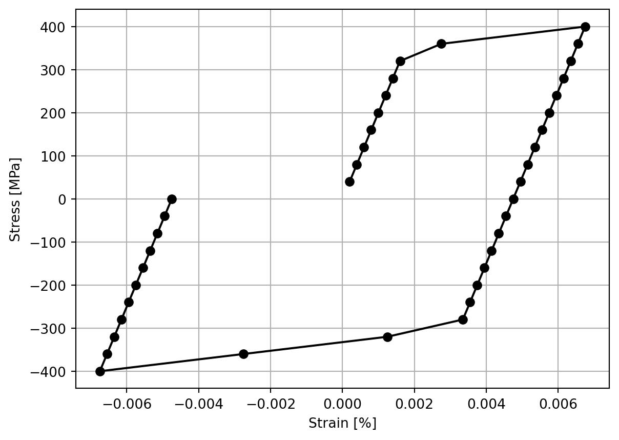
8.5.2 Response Statistics
The second-moment information provided in Listing 8.14 is employed here, in conjunction with first- and second-order response sensitivities to calculate the second-order mean and first-order variance given by Equation 4.12 and Equation 4.13, respectively:
covarianceMatrix = getCovMatrix(means, stdvs, correlation)
meanSO = np.copy(u)
for n in range(len(t)):
    meanSO[n] += 0.5 * np.sum(Hessian[:,:,n] * covarianceMatrix)
stdvFO = []
for n in range(len(t)):
    stdvFO.append(np.sqrt(dudx[:,n].dot(covarianceMatrix.dot(dudx[:,n]))))
stdvFO = np.divide(stdvFO, 10)
plt.figure()
plt.fill_betweenx(np.multiply(F*1e-6, lamda), meanSO-stdvFO, meanSO+stdvFO, color='0.8')
plt.plot(u, np.multiply(F*1e-6, lamda), 'k-', markersize=3, label='Response')
plt.plot(meanSO, np.multiply(F*1e-6, lamda), 'r-', label='Second-order mean')
plt.plot(meanSO+stdvFO, np.multiply(F*1e-6, lamda), 'b-', label='$\\pm 0.1 \\cdot \\sigma_u$')
plt.plot(meanSO-stdvFO, np.multiply(F*1e-6, lamda), 'b-')
plt.grid(True)
plt.xlabel("Strain [%]")
plt.ylabel("Stress [MPa]")
plt.legend(loc='upper left')
plt.show()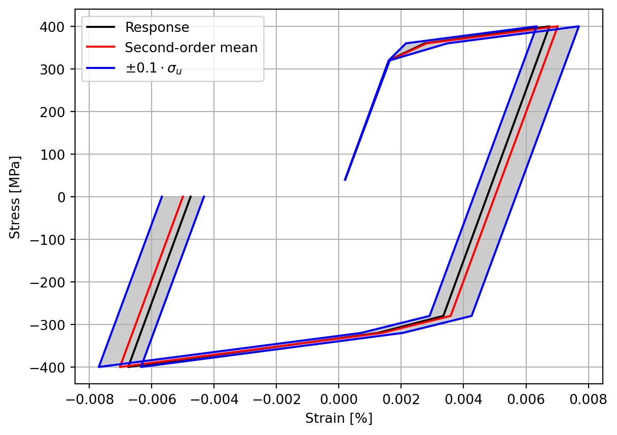
The plot shows that the second-order mean, marked with a red line, is slightly different from the first-order mean, which is the response itself, marked with a black line. However, it is the significant increase in the response standard deviation after yielding that stands out. In fact, to make the plot readable it is necessary to shade only \(\pm 10%\) of the value of that standard deviation. This jump in variance in the nonlinear response region is confirmed by reliability analysis later in this chapter. It is explained by the fact that different outcomes of \(f_y\) lifts or lowers the point of yielding; conversely, the response, \(u=\varepsilon\), is measured along the abscissa axis. Utilizing the stress-strain relationship after yielding, \(\sigma=(\alpha \cdot E) \varepsilon\), we see that a unit change in \(\sigma\) gives a \(\frac{1}{\alpha \cdot E}\) change in the strain. The formulation of the random variable \(f_y\) along the vertical axis with the response \(\varepsilon\) measured along the horizontal contributes to the large response variance after yielding.
8.5.3 First-order Sensitivities
Near the end of Chapter 3, first-order response sensitivities are multiplied with respective standard deviations to make the sensitivity values comparable. That approach is adopted here, with a plot of \(\frac{\partial u}{\partial x_i}\cdot \sigma_i\) created:
plt.figure()
plt.plot(t, u, 'k-', label='$u$')
plt.plot(t, np.multiply(dudx[0, :], stdvs[0]),     'b-', label='$\\frac{\\partial u}{\\partial E}$')
plt.plot(t, np.multiply(dudx[1, :], stdvs[1]),    'r-', label='$\\frac{\\partial u}{\\partial f_y}$')
plt.plot(t, np.multiply(dudx[2, :], stdvs[2]), 'g-', label='$\\frac{\\partial u}{\\partial \\alpha}$')
plt.grid(True)
plt.xlabel("Pseudo time")
plt.legend(loc='upper left')
plt.show()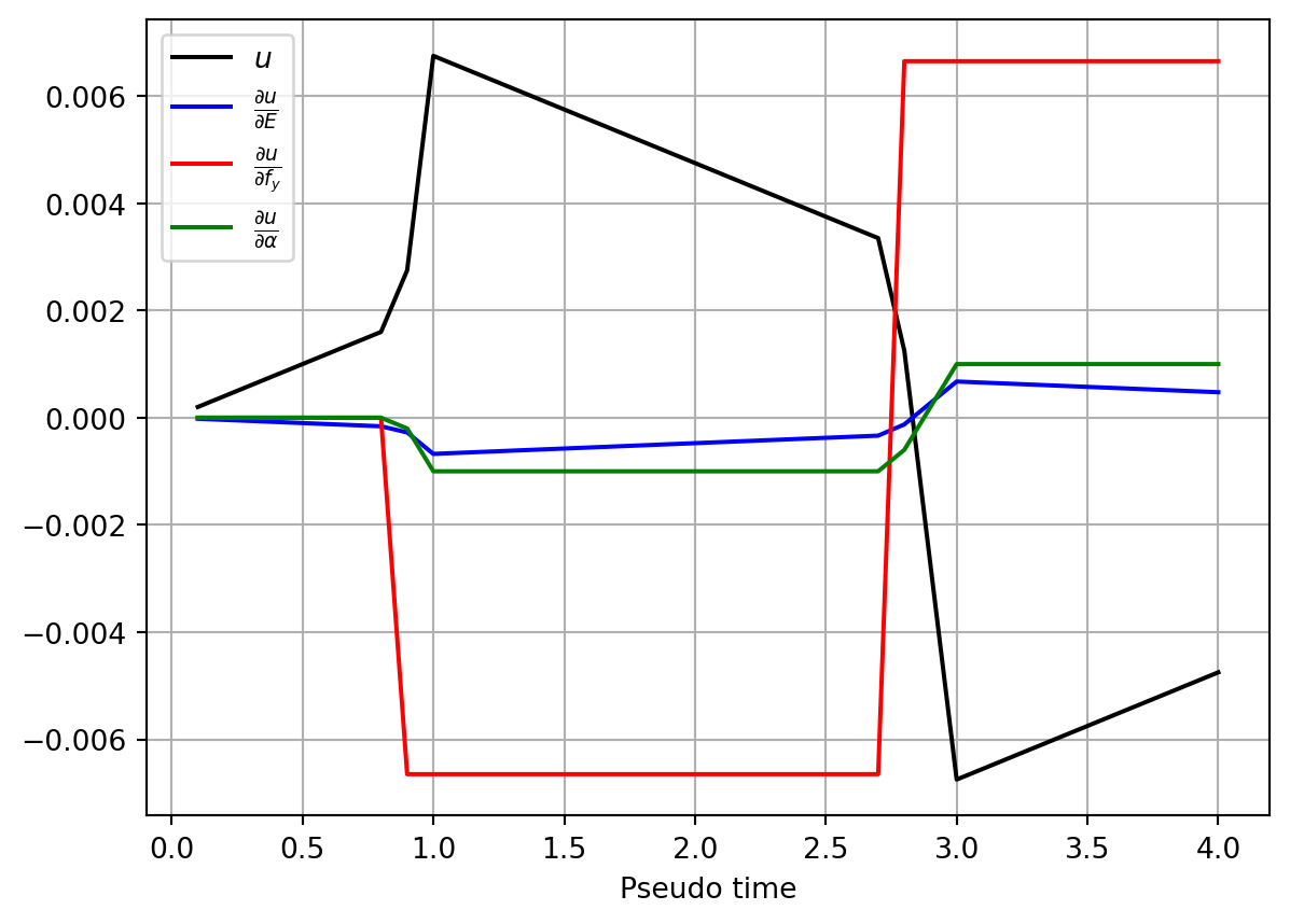
We see that the sensitivity with respect to the yield stress, \(f_y\), is overall largest, but only after yielding. In fact, a 20% change in the value of \(f_y\), as per the previously given covfy value, would according to \(\frac{\partial u}{\partial x_i}\) lead to a response change in the order of the original displacement response.
8.5.4 Second-order Sensitivities
Now considering \(\frac{\partial^2 u}{\partial x_i \partial x_j}\cdot \sigma_i \cdot \sigma_j\), the results shown below reveals that the cross-derivatives between \(f_y\) and \(\alpha\), and also between \(f_y\) and \(E\) are most significant, but again only after yielding:
plt.figure()
plt.plot(t, np.multiply(Hessian[0, 0, :], stdvs[0]*stdvs[0]), 'r-',     label='$\\frac{\\partial^2 u}{\\partial E \\partial E}$')
plt.plot(t, np.multiply(Hessian[0, 1, :], stdvs[0]*stdvs[1]), 'g-',    label='$\\frac{\\partial^2 u}{\\partial E \\partial f_y}$')
plt.plot(t, np.multiply(Hessian[0, 2, :], stdvs[0]*stdvs[2]), 'b-', label='$\\frac{\\partial^2 u}{\\partial E \\partial \\alpha}$')

plt.plot(t, np.multiply(Hessian[1, 1, :], stdvs[1]*stdvs[1]), 'm-',    label='$\\frac{\\partial^2 u}{\\partial f_y \\partial f_y}$')
plt.plot(t, np.multiply(Hessian[1, 2, :], stdvs[1]*stdvs[2]), 'y-', label='$\\frac{\\partial^2 u}{\\partial f_y \\partial \\alpha}$')

plt.plot(t, np.multiply(Hessian[2, 2, :], stdvs[2]*stdvs[2]), 'r--', label='$\\frac{\\partial^2 u}{\\partial \\alpha \\partial \\alpha}$')

plt.grid(True)
plt.xlabel("Pseudo time")
plt.legend(loc='upper left')
plt.show()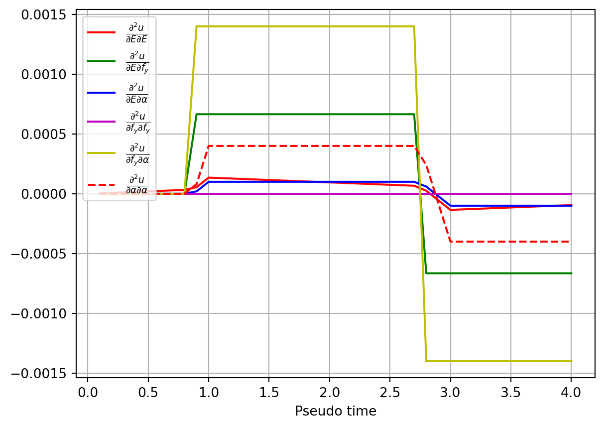
8.5.5 First-order Reliability
Cyclic loading is now ignored, running the structural analysis up to a maximum of \(t=1\). That means unloading is excluded, making the analysis akin to what is called pushover analysis in earthquake engineering. At first, elastic response is considered by taking five steps up to \(t=0.5\). That implies loading up to a stress of \(\sigma=200\)MPa. At that point, response statistics are first calculated:
input = createSingleTrussInput(*means)
structuralModel = model(input)
nsteps = 5
void, void, u, dudx, Hessian = nonlinearStaticAnalysis(structuralModel, nsteps, 0.1, trackNode, trackDOF, DDMs, 2)
meanSO = u[nsteps-1] + 0.5 * np.sum(Hessian[:, :, nsteps-1] * covarianceMatrix)
stdvFO = np.sqrt(dudx[:,nsteps-1].dot(covarianceMatrix.dot(dudx[:,nsteps-1])))
print(f"Response mean={meanSO:.5f}, stdv.={stdvFO:.6f}, c.o.v.={(100*stdvFO/meanSO):.2f}%")
Response mean=0.00101, stdv.=0.000100, c.o.v.=9.90%The corresponding limit-state function makes use of variables defined earlier in this chapter:
def oneTrussHalfLoadLSF(x, threshold, needGradient=True):
    void, void, void, void, trackNode, trackDOF, DDMs = singleTrussVariableSpecs()
    input = createSingleTrussInput(*x)
    structuralModel = model(input)
    nsteps = 5
    dt = 0.1
    if needGradient:
        void, void, u, dudx, void = nonlinearStaticAnalysis(structuralModel, nsteps, dt, trackNode, trackDOF, DDMs, 1)
    else:
        void, void, u, dudx, void = nonlinearStaticAnalysis(structuralModel, nsteps, dt, trackNode, trackDOF)

    return (threshold-u[-1]), -dudx[:, -1]
Reliability analyses are now run for different thresholds, essentially providing a sense of the probability distribution for the response, via the reliability index \(\beta\):
plt.figure()
for c in np.linspace(1, 5, 20):
    threshold = meanSO + c * stdvFO
    beta, xStar, yStar, kappa = iHLRFalgorithm(oneTrussHalfLoadLSF, threshold, means, stdvs, correlation, distributions, basicTransformation, True, False)
    plt.plot(np.multiply(threshold, 100), beta, 'ko', markersize=3)
plt.xlabel("Response threshold (strain in %)")
plt.ylabel("$\\beta$")
plt.grid(True)
plt.show()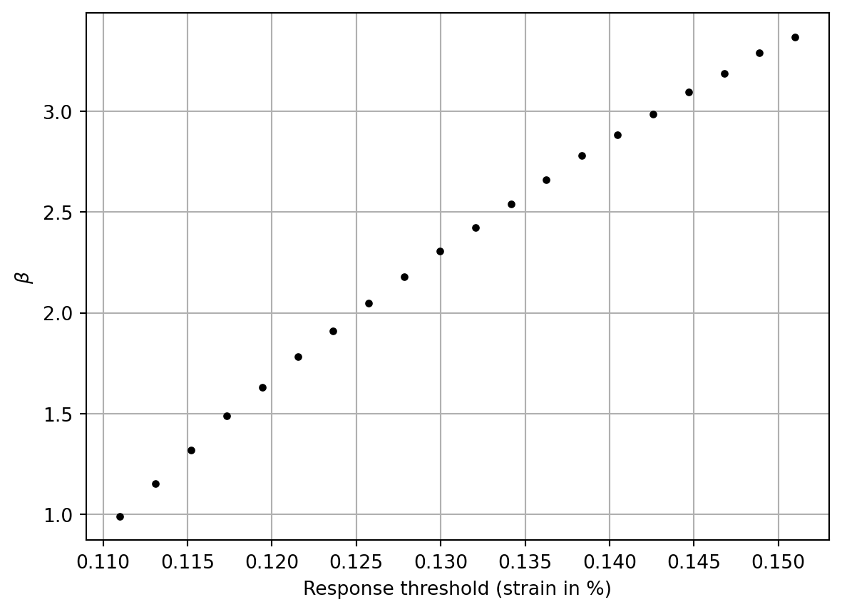
Note that the strain is multiplied by 100 to make the abscissa axis more readable. The plot above shows that the probability of exceeding the threshold “mean plus \(c\) times the standard deviation” goes down as \(c\) increases. A similar observation was made in Chapter 5 for the linear portal frame. Next, we contrast that with pushing the stress up to \(\sigma=400\)MPa. The first hysteretic response plot provided earlier in this chapter says that yielding will now occur. Here is the limit-state function for that case:
def oneTrussFullLoadLSF(x, threshold, needGradient=True):
    void, void, void, void, trackNode, trackDOF, DDMs = singleTrussVariableSpecs()
    input = createSingleTrussInput(*x)
    structuralModel = model(input)
    nsteps = 10
    dt = 0.1
    if needGradient:
        void, void, u, dudx, void = nonlinearStaticAnalysis(structuralModel, nsteps, dt, trackNode, trackDOF, DDMs, 1)
    else:
        void, void, u, dudx, void = nonlinearStaticAnalysis(structuralModel, nsteps, dt, trackNode, trackDOF)
    return (threshold-u[-1]), -dudx[:, -1]
Again, the response statistics are calculated. This time, because of the nonlinear response and resulting large response standard deviation, we observe a 100% coefficient of variation:
input = createSingleTrussInput(*means)
structuralModel = model(input)
nsteps = 10
dt = 0.1
void, void, u, dudx, Hessian = nonlinearStaticAnalysis(structuralModel, nsteps, 0.1, trackNode, trackDOF, DDMs, 1)
meanSO = u[nsteps-1] + 0.5 * np.sum(Hessian[:, :, nsteps-1] * covarianceMatrix)
stdvFO = np.sqrt(dudx[:,nsteps-1].dot(covarianceMatrix.dot(dudx[:,nsteps-1])))
print(f"Response mean={meanSO:.5f}, stdv.={stdvFO:.6f}, c.o.v.={(100*stdvFO/meanSO):.2f}%")
Response mean=0.00675, stdv.=0.006759, c.o.v.=100.13%The result of running reliability analysis with the oneTrussFullLoadLSF() limit-state function defined above is:
plt.figure()
for c in np.linspace(1, 5, 20):
    threshold = meanSO + c * stdvFO
    beta, xStar, yStar, kappa = iHLRFalgorithm(oneTrussFullLoadLSF, threshold, means, stdvs, correlation, distributions, basicTransformation, True, False)
    plt.plot(threshold, beta, 'ko', markersize=3)
plt.xlabel("Response threshold (strain)")
plt.ylabel("$\\beta$")
plt.grid(True)
plt.show()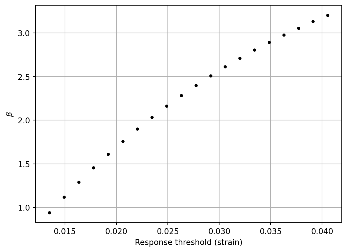
Comparing the abscissa axis of the two previous plots confirms the significantly larger variance in the nonlinear response range.
8.5.6 Second-order Reliability
The previous plot shows that the reliability index associated with exceeding the limit 0.035 is slightly below 3.0. However, the basic probability transformation is utilized above, meaning the probability distribution types given in Listing 8.14 are not accounted for. Now, the iHLRF algorithm is rerun at that response threshold with the Nataf probability transformation, in preparation for SORM analysis, which does indeed account for distribution types:
threshold = 0.035
beta, xStar, yStar, kappa = iHLRFalgorithm(oneTrussFullLoadLSF, threshold, means, stdvs, correlation, distributions, natafTransformation, False, True)
HLRF step 1: Check1=1.00e+00,Check2=0.00e+00, y-norm=1.000
HLRF step 2: Check1=1.53e-01,Check2=7.63e-01, y-norm=4.058
HLRF step 3: Check1=2.10e-01,Check2=4.63e-01, y-norm=3.176
HLRF step 4: Check1=9.93e-02,Check2=2.77e-01, y-norm=3.333
HLRF step 5: Check1=9.36e-03,Check2=1.08e-01, y-norm=3.502
HLRF step 6: Check1=4.58e-03,Check2=5.96e-02, y-norm=3.505
HLRF step 7: Check1=1.14e-03,Check2=3.06e-02, y-norm=3.511
HLRF step 8: Check1=3.52e-04,Check2=1.67e-02, y-norm=3.513
HLRF step 9: Check1=9.74e-05,Check2=8.85e-03, y-norm=3.513
iHLRF algorithm converged with beta=3.513We see that the FORM analysis converges in 9 steps without use of the golden section search for the optimal step size at each iHLRF iteration. In offline analyses it is observed that 5 steps are needed if that search is conducted, but that increases the total number of evaluations of the limit-state function. We also observe that the introduction of the Lognormal probability distribution for the random variables has an effect. While the previous plot shows a reliability index below 3.0 at the given response threshold, the reliability index is now in excess of 3.5. Next, a SORM analysis is conducted at the same response threshold:
input = createSingleTrussInput(*xStar)
structuralModel = model(input)
nsteps = 10
dt = 0.1
void, void, void, dudx, xHessian = nonlinearStaticAnalysis(structuralModel, nsteps, dt, trackNode, trackDOF, DDMs, 2)
pfFORM, pfSORM, curvatures = SORM(beta, xStar, yStar, dudx[:,-1], xHessian[:,:,-1], means, stdvs, correlation, distributions)
FORM failure probability: 0.00022 (Reliability index 3.513)
SORM failure probability: 0.00018 (Reliability index 3.569, from pf)We see that the SORM result further reduces the failure probability, in this case. The correction of the FORM result is not dramatic, but the analysis demonstrates the value of complementing FORM with SORM for problems with significant nonlinearity.