from Chapter5code import *6 Nataf and SORM
The title of this chapter is cryptic for readers unfamiliar with reliability methods. Nataf refers to a probability transformation that accounts for both correlation and marginal probability distributions for the random variables. The techniques developed in the previous chapter did not employ the full distributions, only second-moment information for the random variables, producing the reliability index, \(\beta\), without taking the step to a failure probability. Except the simple case of Normal random variables, that step is what the Nataf transformation facilitates.
SORM is the acronym for the second-order reliability method. The FOSM method from the previous chapter is a first-order method, as the two first letters in its abbreviation suggest. The extension of FOSM to include probability distributions while sticking with the first-order Taylor approximation of the limit-state function is historically labelled FORM, i.e., the first-order reliability method. It is in that light that SORM is a natural acronym, enhancing FORM with a second-order Taylor approximation of the limit-state function.
The material presented in this chapter can be labelled advanced reliability methods. That is because it is extending the methods from the previous chapter, without necessarily being employed by all readers. Furthermore, Nataf and SORM are independent techniques. The Nataf transformation is used to include probability distributions in reliability analysis, when correlation is present, regardless of whether SORM is employed. Conversely, SORM extends the FOSM analysis from the previous chapter, without necessarily employing the Nataf transformation. However, SORM without Nataf is a special case, with the Normal distribution implied. That is because SORM does not provide \(\beta\), it provides \(p_f\).
6.1 Nataf Transformation
In the previous chapter, Equation 5.7 and Equation 5.15 are utilized to transform the original \(\mathbf{x}\) random variables into the Standard \(\mathbf{y}\) space. The latter of those equations accounts for correlation, but none of them employ the probability distribution for the \(\mathbf{x}\) variables.
When probability distributions are introduced, the \(\mathbf{y}\) space of takes on a new meaning. It now becomes the Standard Normal space, meaning that the \(\mathbf{y}\) variables have the Normal distribution, still uncorrelated with zero mean and unit variance. The multivariate Normal PDF for the \(\mathbf{y}\) variables reads
\[ \varphi(\mathbf{y}) = \frac{1}{\sqrt{(2\pi)^N}} \cdot \exp\left(-\frac{1}{2} \mathbf{y}^{\top}\mathbf{y}\right) \] {eq-joint-standard-normal}
where \(N=\) number of random variables. More important than the expression is the property that the probability content outside a hyper-plane in the \(\mathbf{y}\) space with distance \(\beta\) from the origin is
\[ p_f = \Phi (-\beta) \tag{6.1}\]
This means that Equation 5.2 remains valid, with \(\beta\) from Equation 5.19, further motivating the use of the \(\mathbf{y}\) space and the Nataf transformation in the face of prescribed probability distributions. The Nataf transformation between \(\mathbf{x}\) and \(\mathbf{y}\) employs a set of auxiliary and Normal variables, \(\mathbf{z}\), with the transformation process outlined as follows:
- \(\mathbf{x} \Longleftrightarrow\mathbf{z}\)
- \(\mathbf{z} \Longleftrightarrow\mathbf{y}\)
The step between \(\mathbf{x}\) and \(\mathbf{z}\) is addressed first. This step accounts for the probability distributions but ignores correlation. This step is done one random variable at a time, using what statisticians refer to as the probability preserving transformation:
\[ \Phi(z) = F(x) \tag{6.2}\]
That transformation intuitively expresses, via two CDFs, that the \(z\) value that corresponds to an \(x\) value has the same probability of of not being exceeded. Solving Equation 6.2 gives the first part of the Nataf transformation:
\[ z = \Phi^{-1}\left(F(x)\right) \Longleftrightarrow x = F^{-1}\left(\Phi(z)\right) \tag{6.3}\]
The individual \(z\) variables are now Normal. The fundamental assumption in the Nataf transformation, developed by Liu and Der Kiureghian (1986), is that they are jointly Normal. Because they have zero mean and unit variance, the following version of Equation 5.15 takes correlation into account:
\[ \mathbf{y} = \mathbf{L}^{-1} \mathbf{z} \Longleftrightarrow \mathbf{z} = \mathbf{L} \mathbf{y} \tag{6.4}\]
6.1.1 Modified Correlation Matrix
An issue with Equation 6.4 is that the Cholesky matrix, \(\mathbf{L}\), is not the decomposition of the correlation matrix for the original \(\mathbf{x}\) variables. That is because the correlation between the \(\mathbf{z}\) variables is not the same as the correlation between the \(\mathbf{x}\) variables. The relationship between two correlation coefficients is
\[ \rho_{ij} = \int_{-\infty}^{\infty} \left( \frac{x_i - \mu_i}{\sigma_i} \right) \left( \frac{x_j - \mu_j}{\sigma_j} \right) \cdot \varphi_2(z_i, z_j, \tilde{\rho}_{ij}) \,dz_i \,dz_j \tag{6.5}\]
where \(\rho_{ij}=\) correlation between \(x_i\) and \(x_j\), \(\tilde{\rho}_{ij}=\) correlation between \(z_i\) and \(z_j\), and the bivariate Standard Normal PDF is
\[ \varphi_2(z_i, z_j, \tilde{\rho}_{ij}) = \frac{1}{2 \pi \sqrt{1-\tilde{\rho}_{ij}}} \mathrm{exp}\left(- \frac{z_i^2 + z_j^2 - 2 \cdot \tilde{\rho}_{ij} \cdot z_i \cdot z_j}{2 \cdot (1-\tilde{\rho}^2_{ij})} \right) \tag{6.6}\]
With the understanding that \(\mathbf{L}\) in Equation 6.4 is the Cholesky decomposition of the correlation matrix containing the coefficients \(\tilde{\rho}_{ij}\), the Nataf transformation is now complete. Liu and Der Kiureghian (1986) developed formulas for \(\tilde{\rho}_{ij}\) from \(\rho_{ij}\) for different distribution types. Some of them, covering the Normal, Lognormal, and Uniform distribution types are implemented here:
def modifyCorrelationMatrix(means, stdvs, distributions, correlation):
    numRV = len(means)
    modifiedR = np.identity(numRV)
    correlation = np.array(correlation)
    for i in range(len(correlation)):
        rv_i = int(correlation[i, 0])
        rv_j = int(correlation[i, 1])
        rho_original = correlation[i, 2]
        mean_i = means[rv_i - 1]
        mean_j = means[rv_j - 1]
        stdv_i = stdvs[rv_i - 1]
        stdv_j = stdvs[rv_j - 1]
        distr_i = distributions[rv_i - 1]
        distr_j = distributions[rv_j - 1]
        if distr_i == "Normal" and distr_j == "Normal":
            rho_new = rho_original
        elif distr_i == "Lognormal" and distr_j == "Lognormal":
            cov_i = stdv_i / mean_i
            cov_j = stdv_j / mean_j
            rho_new = np.log(1+rho_original*cov_i*cov_j) / np.sqrt(np.log(1+cov_i**2) * np.log(1+cov_j**2))
        elif distr_i == "Uniform" and distr_j == "Uniform":
            C = 1.047 - 0.047 * rho_original**2
            rho_new = C * rho_original
        elif (distr_i == "Normal" and distr_j == "Uniform") or (distr_i == "Uniform" and distr_j == "Normal"):
            C = 1.023
            rho_new = C * rho_original
        elif distr_i == "Normal" and distr_j == "Lognormal":
            cov = stdv_j / mean_j
            C = cov / np.sqrt(np.log(1+cov**2))
            rho_new = C * rho_original
        elif distr_i == "Lognormal" and distr_j == "Normal":
            cov = stdv_i / mean_i
            C = cov / np.sqrt(np.log(1+cov**2))
            rho_new = C * rho_original
        elif distr_i == "Lognormal" and distr_j == "Uniform":
            cov = stdv_i / mean_i
            C = 1.019 + 0.014*cov + 0.01*rho_original**2 + 0.249 * cov**2
            rho_new = C * rho_original
        elif distr_i == "Uniform" and distr_j == "Lognormal":
            cov = stdv_j / mean_j
            C = 1.019 + 0.014*cov + 0.01*rho_original**2 + 0.249 * cov**2
            rho_new = C * rho_original
        modifiedR[rv_i-1, rv_j-1] = rho_new
        modifiedR[rv_j-1, rv_i-1] = rho_new
    return modifiedR
That function is soon applied in an updated version of the basic probability transformation in Listing 5.1.
6.1.2 Jacobian
While reliability analysis is conducted in the \(\mathbf{y}\) space, the limit-state function and its gradient are evaluated from structural analyses in the original \(\mathbf{x}\) space. That is why the chain rule of differentiation was applied in Section 5.5 to obtain \(\frac{\partial G}{\partial \mathbf{y}}\) from \(\frac{\partial g}{\partial \mathbf{x}}\).
That passage in the previous chapter shows that the Jacobian matrix \(\frac{\partial \mathbf{x}}{\partial \mathbf{y}}\) is needed. Given the developments above, the Jacobian of the transformation is now a bit more involved than the derivative \(\frac{\partial \mathbf{x}}{\partial \mathbf{y}}=\mathbf{DL}\) that appeared in the previous chapter.
Because Nataf is a two-step transformation, the Jacobian is here formed in two steps. First, Equation 6.2 is differentiated with respect to \(z\):
\[ \varphi(z) = \frac{\partial}{\partial z} F(x) = \frac{\partial x}{\partial z} \frac{\partial}{\partial x}F(x) = \frac{\partial x}{\partial z}f(x) \tag{6.7}\]
That shows the Jacobian is the ratio of the PDFs: \(\frac{\partial x}{\partial z}=\frac{\varphi(z)}{f(x)}\). Next, we add the second step of the Nataf transformation from Equation 6.4 to obtain the sought result:
\[ \frac{\partial \mathbf{x}}{\partial \mathbf{y}} = \frac{\partial \mathbf{x}}{\partial \mathbf{z}}\frac{\partial \mathbf{z}}{\partial \mathbf{y}} = \mathrm{diag}\left[ \frac{\varphi(z_i)}{f(x_i)}\right] \mathbf{L} \tag{6.8}\]
That Jacobian, with a square diagonal matrix identified, is now implemented along with the rest of the Nataf transformation.
6.1.3 Implementation
def natafTransformation(y, means, stdvs, correlation, distributions):
    from scipy.stats import norm, uniform
    if len(correlation)==0 and len(distributions)==0:
        x = means + np.dot(np.diag(stdvs), y)
        dxdy = np.diag(stdvs)
    elif len(correlation) > 0 and len(distributions)==0:
        R = getR(means, correlation)
        L = np.linalg.cholesky(R)
        x = means + np.dot(np.dot(np.diag(stdvs), L), y)
        dxdy = np.dot(np.diag(stdvs), L)
    else:
        numRVs = len(means)
        if len(correlation) > 0:
            modifiedR = modifyCorrelationMatrix(means, stdvs, distributions, correlation)
            L = np.linalg.cholesky(modifiedR)
        else:
            L = np.identity(numRVs)
        z = L.dot(y)
        x = np.zeros(numRVs)
        dxdz = np.zeros((numRVs, numRVs))
        for j in range(numRVs):
            if distributions[j] == "Normal":
                x[j] = z[j] * stdvs[j] + means[j]
                dxdz[j, j] = stdvs[j]
            elif distributions[j] == "Lognormal":
                mu = np.log(means[j]) - 0.5 * np.log(1 + (stdvs[j] / means[j]) * (stdvs[j] / means[j]))
                sigma = np.sqrt(np.log((stdvs[j] / means[j]) * (stdvs[j] / means[j]) + 1))
                x[j] = np.exp(z[j] * sigma + mu)
                dxdz[j, j] = sigma * np.exp(z[j] * sigma + mu)
            elif distributions[j] == "Uniform":
                halfspan = np.sqrt(3) * stdvs[j]
                a = means[j] - halfspan
                x[j] = uniform.ppf(norm.cdf(z[j]), a, 2*halfspan)
                f = uniform.pdf(x[j], a, 2 * halfspan)
                phi = norm.pdf(z[j])
                dxdz[j, j] = phi / f
        dxdy = dxdz.dot(L)
    return x, dxdy
The Nataf transformation implemented above is now tested for the linear frame analyzed in previous chapters. That means we employ the Lognormal probability distribution specified for the random variables in Listing 3.6. The result is a reliability index slightly different from that calculated in Chapter 5:
means, stdvs, distributions, correlation, trackNode, trackDOF, DDMs = linearFrameVariableSpecs()
beta, xStar, yStar, kappa = iHLRFalgorithm(linearFrameLSF, 0.025, means, stdvs, correlation, distributions, natafTransformation, False)
HLRF step 1: Check1=1.00e+00,Check2=0.00e+00, y-norm=1.000
HLRF step 2: Check1=3.22e-01,Check2=3.65e-04, y-norm=2.470
HLRF step 3: Check1=1.57e-02,Check2=5.28e-05, y-norm=2.004
HLRF step 4: Check1=4.26e-05,Check2=6.21e-06, y-norm=1.979
iHLRF algorithm converged with beta=1.9796.2 Second-order Reliability Method
The reliability method presented in Chapter 5 is called first-order because of the Taylor linearization in Equation 5.22. In an iterative approach, that approximation was enforced repeatedly at trial points in the \(\mathbf{y}\) space, until the design point was determined. That point, denoted by \(\mathbf{y}^*\), was employed in Equation 5.19 to determine the reliability index, \(\beta\). Emphasis was placed on \(\beta\) as a proxy for reliability, without taking the step to calculate the failure probability, \(p_f\). Now, building upon the introduction of probability distributions above, that step is taken. This starts with a second-order Taylor approximation of the limit-state function at \(\mathbf{y}^*\):
\[ G(\mathbf{x}) \approx \nabla G^{\top} (\mathbf{y}-\mathbf{y}^*) + \frac{1}{2} (\mathbf{y}-\mathbf{y}^*)^{\top} \mathbf{H} (\mathbf{y}-\mathbf{y}^*) \tag{6.9}\]
\(G(\mathbf{y}^*)\) is omitted because the value of the limit-state function is zero at the design point. The gradient vector, \(\nabla G \equiv \frac{\partial G}{\partial y_i}\), and Hessian matrix, \(\mathbf{H} \equiv \frac{\partial^2 G}{\partial y_i \partial y_j}\), are evaluated at \(\mathbf{y}^*\).
With the approximation in Equation 6.9 we can, according to Breitung (1984), express the failure probability as a correction of the first-order version in Equation 6.1:
\[ p_f \approx \Phi (-\beta) \cdot \prod\limits_{i=1}^{N-1} \frac{1}{\sqrt{1+ \beta \cdot \kappa_i}} \tag{6.10}\]
where \(\kappa_i=\) curvature number \(i\) of the limit-state function at the design point. Notice that there is one less curvature than there are random variables. We also observe that no new iterative search is needed to obtain the second-order estimate of \(p_f\). However, the search for \(\mathbf{y}^*\) must precede the evaluation of Equation 6.10.
6.2.1 Curvatures from Hessian
One way to get the curvatures needed for the evaluation of Equation 6.10 is to utilize the exact second-order response sensitivities calculated in Chapter 3. From that chapter we have both the gradient vector, \(\frac{\partial u}{\partial x_i}\), and the Hessian matrix, \(\frac{\partial^2 u}{\partial x_i \partial x_j}\), in the \(\mathbf{x}\) space. Because reliability anlaysis takes place in the \(\mathbf{y}\) space, the chain rule of differentiation was applied in Section 5.5 to get the gradient vector in the \(\mathbf{y}\) space.
The same needs to be done for the Hessian. To provide a basis for the derivations, the transformation of the gradient vector is now written in index notation:
\[ \frac{\partial G}{\partial y_j} = \frac{\partial g}{\partial u_k}\frac{\partial u_k}{\partial x_m}\frac{\partial x_m}{\partial y_j} \tag{6.11}\]
That equation is differentiated once again to obtain the transformation of the Hessian from the \(\mathbf{x}\) space to the \(\mathbf{y}\) space. Notice that the product rule of differentiation is employed to differentiate Equation 6.11, giving three terms, each with a square bracket that in turn applies the chain rule of differentiation:
\[ \begin{aligned} \frac{\partial^2 G}{\partial y_i \partial y_j} &= \frac{\partial}{\partial y_i} \left(\frac{\partial g}{\partial u_k}\frac{\partial u_k}{\partial x_m}\frac{\partial x_m}{\partial y_j} \right) \\ &= \left[ \frac{\partial^2 g}{\partial u_k \partial u_p} \frac{\partial u_p}{\partial x_q} \frac{\partial x_q}{\partial y_i} \right] \frac{\partial u_k}{\partial x_m}\frac{\partial x_m}{\partial y_j} \\ &+ \frac{\partial g}{\partial u_k} \left[ \frac{\partial^2 u_k}{\partial x_m \partial x_q} \frac{\partial x_q}{\partial y_i} \right] \frac{\partial x_m}{\partial y_j} \\ &+ \frac{\partial g}{\partial u_k}\frac{\partial u_k}{\partial x_m}\left[\frac{\partial^2 x_m}{\partial y_i \partial y_j}\right] \end{aligned} \tag{6.12}\]
That equation is similar to Equation 3 in the paper by Bebamzadeh and Haukaas (2008). The first term after the equal sign is zero because \(\frac{\partial^2 g}{\partial u_k \partial u_p}=0\). The second term contains the second-order derivative calculated alongside the structural response and first-order sensitivities in this book. The third term contains the “second-order Jacobian” of the probability transformation, i.e., \(\frac{\partial^2 x_m}{\partial y_j \partial y_i}\). To obtain it, the ordinary Jacobian resulting from Equation 6.7 is now differentiated with respect to another \(z\) variable. However, because that result is a diagonal matrix, as seen in Equation 6.8, we can skip index notation for brevity, focusing on the diagonal terms:
\[ \begin{aligned} \frac{\partial^2 x}{\partial z^2} &= \frac{\partial}{\partial z} \left(\frac{\varphi(z)}{f(x)}\right) \\ &= \frac{\partial \varphi(z)}{\partial z} \frac{1}{f(x)} + \frac{\partial}{\partial z} \left(\frac{1}{f(x)}\right)\varphi(z) \\ &= \frac{\partial \varphi(z)}{\partial z} \frac{1}{f(x)} + \frac{\partial}{\partial x} \left(\frac{1}{f(x)}\right)\frac{\partial x}{\partial z}\varphi(z) \\ &= \frac{\partial \varphi(z)}{\partial z} \frac{1}{f(x)} - \frac{1}{f(x)^2}\frac{\partial f(x)}{\partial x} \frac{\partial x}{\partial z}\varphi(z) \end{aligned} \tag{6.13}\]
In order to bring in the \(\mathbf{z}\) variables and obtain \(\frac{\partial^2 x_m}{\partial y_j \partial y_i}\), and ultimately substitute the result into Equation 6.12, it is helpful to return to index notation. In doing so, we remember that dummy indices, i.e., those appearing twice in a term with summation implied, can be casually renamed, as long as the same symbol is not used in the same term:
\[ \begin{aligned} \frac{\partial^2 x_m}{\partial y_i \partial y_j} &= \frac{\partial }{\partial y_i}\left(\frac{\partial x_m}{\partial y_j}\right) \\ &= \frac{\partial }{\partial y_i}\left(\frac{\partial x_m}{\partial z_p}\frac{\partial z_p}{\partial y_j}\right) \\ &= \frac{\partial }{\partial y_i}\left(\frac{\partial x_m}{\partial z_p}\frac{\partial z_p}{\partial y_j}\right) + \frac{\partial }{\partial y_i}\left(\frac{\partial x_m}{\partial z_p}\frac{\partial z_p}{\partial y_j}\right) \\ &= \frac{\partial^2 x_m}{\partial z_p \partial z_p}\frac{\partial z_p}{\partial y_i} \frac{\partial z_p}{\partial y_j} + \frac{\partial x_m}{\partial z_p}\frac{\partial^2 z_p}{\partial y_i \partial y_j} \\ \end{aligned} \tag{6.14}\]
The first term in that result utilizes the derivation in Equation 6.13. The last term is zero because \(\mathbf{L}\) does not vary with \(\mathbf{y}\). The derivative of \(\mathbf{z}\) with respect to \(\mathbf{y}\) is that Cholesky matrix. What that in mind, we can further refine Equation 6.14:
\[ \frac{\partial^2 x_m}{\partial y_i \partial y_j} = \left[ \frac{\partial \varphi(z)}{\partial z} \frac{1}{f(x)} - \frac{1}{f(x)^2}\frac{\partial f(x)}{\partial x} \frac{\partial x}{\partial z}\varphi(z) \right]_{mpo} L_{pi}L_{oj} \tag{6.15}\]
Substitution of that equation as well as Equation 6.8 into Equation 6.12 gives the final expression for the Hessian in the Standard Normal space as a function of the exact second-order response sensitivities calculated in Chapter 3:
\[ \begin{aligned} \frac{\partial^2 G}{\partial y_i \partial y_j} &= \frac{\partial g}{\partial u_k} \left[ \frac{\partial^2 u_k}{\partial x_m \partial x_q} \frac{\partial x_q}{\partial y_i} \right] \frac{\partial x_m}{\partial y_j} \\ &+ \frac{\partial g}{\partial u_k}\frac{\partial u_k}{\partial x_m}\left[\frac{\partial^2 x_m}{\partial y_i \partial y_j}\right] \\ &= \frac{\partial g}{\partial u_k} \left[ \frac{\partial^2 u_k}{\partial x_m \partial x_q} \cdot \mathrm{diag}\left[ \frac{\varphi(z)}{f(x)}\right]_{qo} L_{oi} \right] \cdot \mathrm{diag}\left[ \frac{\varphi(z)}{f(x)}\right]_{mp} L_{pj} \\ &+ \frac{\partial g}{\partial u_k}\frac{\partial u_k}{\partial x_m}\cdot \mathrm{diag}\left[ \frac{\partial \varphi(z)}{\partial z} \frac{1}{f(x)} - \frac{1}{f(x)^2}\frac{\partial f(x)}{\partial x} \frac{\partial x}{\partial z}\varphi(z) \right]_{mpo} L_{pi}L_{oj} \\ &= \frac{\partial g}{\partial u_k} \frac{\partial^2 u_k}{\partial x_m \partial x_q} \left[ \frac{\partial x}{\partial z}\right]_{q} L_{qi} \left[ \frac{\partial x}{\partial z}\right]_{m} L_{mj} \\ &+ \frac{\partial g}{\partial u_k}\frac{\partial u_k}{\partial x_m}\left[ \frac{\partial \varphi(z)}{\partial z} \frac{1}{f(x)} - \frac{1}{f(x)^2}\frac{\partial f(x)}{\partial x} \frac{\partial x}{\partial z}\varphi(z) \right]_{m} L_{mi}L_{mj} \end{aligned} \tag{6.16}\]
Summation is now implied also for dummy indices that appear three times in a term. In the last equality above, some dummy indices are removed to take advantage of the diagonality of the \(\varphi/f\) matrices and the third-order tensor in square brackets in Equation 6.15. Also in the last equality, the substitution \(\frac{\partial x}{\partial z} \equiv \frac{\varphi(z)}{f(x)}\) from Equation 6.8 is made to make the expression more readable.
A statement known from the field of optimization analysis is that the Hessian should be a pure expression of curvature, not influenced by the gradient of the limit-state function at \(\mathbf{y}^*\). For that reason, the Hessian from Equation 6.16 is normalized by the norm of the gradient. That is done in the SORM algorithm presented shortly. First, here is the function that calculates the Hessian in the Standard Normal space from second-order response sensitivities from structural analysis:
def transformHessian(xStar, xGradient, xHessian, means, stdvs, correlation, distributions):
    numRVs = len(means)
    from scipy.stats import norm, lognorm, uniform
    dxdz = []
    bracket = []
    for i in range(numRVs):
        x = xStar[i]
        if distributions[i] == 'Normal':
            z = norm.ppf(norm.cdf(x))
            phi = norm.pdf(z)
            f = norm.pdf(x, means[i], stdvs[i])
            dxdz.append(phi/f)
            dphidz = -z * norm.pdf(z)
            dfdx = -(x-means[i])/stdvs[i]**2 * norm.pdf(x, means[i], stdvs[i])
            bracket.append(dphidz/f - dfdx/f**2 * phi**2/f)
        elif distributions[i] == 'Lognormal':
            mu = np.log(means[i]) - 0.5 * np.log(1 + (stdvs[i] / means[i]) * (stdvs[i] / means[i]))
            sigma = np.sqrt(np.log((stdvs[i] / means[i]) * (stdvs[i] / means[i]) + 1))
            z = norm.ppf(lognorm.cdf(x, sigma, 0, np.exp(mu)))
            phi = norm.pdf(z)
            f = lognorm.pdf(x, sigma, 0, np.exp(mu))
            dxdz.append(phi/f)
            dphidz = -z * norm.pdf(z)
            dfdx = -f/x * (1 + (np.log(x)-mu)/sigma**2)
            bracket.append(dphidz/f - dfdx/f**2 * phi**2/f)
        elif distributions[i] == 'Uniform':
            halfspan = np.sqrt(3) * stdvs[i]
            a = means[i] - halfspan
            z = norm.ppf(uniform.cdf(x, a, 2*halfspan))
            phi = norm.pdf(z)
            f = uniform.pdf(x, a, 2*halfspan)
            dxdz.append(phi/f)
            dphidz = -z * norm.pdf(z)
            dfdx = 0
            bracket.append(dphidz/f - dfdx/f**2 * phi**2/f)
        if len(correlation) > 0:
            modifiedR = modifyCorrelationMatrix(means, stdvs, distributions, correlation)
            L = np.linalg.cholesky(modifiedR)
        else:
            L = np.identity(numRVs)
    dgdu = -1  # Assumption: g=threshold-u

    term1 = dgdu * np.einsum('mq,q,qi,m,mj->ij', xHessian, dxdz, L, dxdz, L)
    term2 = dgdu * np.einsum('m,m,mi,mj->ij', xGradient, bracket, L, L)
    yHessian = term1 + term2

    return yHessian
That transformation is utilized in the SORM algorithm shown below. As described in Chapter 7 in the book by Der Kiureghian (2022), the \(\mathbf{y}\) coordinate system is rotated such that the last axis direction points in the direction of the \(\pmb{\alpha}\) vector:
def SORM(beta, xStar, yStar, dudx, xHessian, means, stdvs, correlation, distributions):

    # Transform gradient
    void, dxdy = natafTransformation(yStar, means, stdvs, correlation, distributions)
    dgdu = -1
    yGradient = dgdu * dudx.dot(dxdy)
    yGradientNorm = np.linalg.norm(yGradient)
    alpha = -yGradient / yGradientNorm

    # Transform and normalize Hessian
    yHessian = transformHessian(xStar, dudx, xHessian, means, stdvs, correlation, distributions)
    yHessian = yHessian / yGradientNorm

    # Rotation matrix
    numRVs = len(dudx)
    P = np.zeros((numRVs, numRVs))
    P[-1, :] = alpha
    for i in range(numRVs - 1):
        row = np.zeros(numRVs)
        row[i] = 1.0
        for j in range(i):
            row -= np.dot(row, P[j, :]) * P[j, :]
        row -= np.dot(row, alpha) * alpha
        P[i, :] = row / np.linalg.norm(row)

    # Curvatures
    A = np.dot(np.dot(P, yHessian), np.transpose(P))
    Acut = A[:-1, :-1]
    curvatures = np.linalg.eigvals(Acut)

    # Probability estimates
    from scipy.stats import norm
    pfFORM = norm.cdf(-beta)
    SORMcorrection = 1.0
    for i in range(len(curvatures)):
        SORMcorrection *= 1.0 / np.sqrt(1.0 + beta * curvatures[i])
    pfSORM = pfFORM * SORMcorrection
    print(f"FORM failure probability: {pfFORM:.5f} (Reliability index {beta:.3f})")
    print(f"SORM failure probability: {pfSORM:.5f} (Reliability index {-norm.ppf(pfSORM):.3f}, from pf)")
    return pfFORM, pfSORM, curvatures
The label from pf is attached to the reliability index calculated as \(\beta = -\Phi^{-1}(p_{f,SORM})\) from the SORM failure probability. That algorithm is now applied to the portal frame in Figure 1.2. Notice that the structural model is given input values that correspond to the design point found previously by the iHLRF algorithm:
input = createLinearFrameInput(*xStar)
structuralModel = model(input)
void, dudx, xHessian = linearStaticSecondOrder(structuralModel, trackNode, trackDOF, DDMs)
pfFORM, pfSORM, curvatures = SORM(beta, xStar, yStar, dudx, xHessian, means, stdvs, correlation, distributions)
FORM failure probability: 0.02391 (Reliability index 1.979)
SORM failure probability: 0.02430 (Reliability index 1.972, from pf)The result shows a slight correction of the failure probability from the first-order reliability method. The value of the curvatures will be examined in the next subsection.
6.2.2 Curvatures from Design Point Search
A neat approach for approximating the curvatures needed in Equation 6.10 was developed by Der Kiureghian and Stefano (1991). With reference to Figure 6.1, they employed information from the last two trial points in the iHLRF algorithm to determine that curvature by geometrical considerations. From geometry we have that \(\kappa = \frac{1}{R}\), where the radius, \(R\), can be determined from \(\Delta=R\cdot \theta\), where \(\Delta\) is the length of small arc on a circle and \(\theta\) is the angle of the corresponding circle sector. Looking at Figure 6.1, that means
\[ \kappa = \frac{\theta}{\Delta} \approx \frac{\mathrm{cos}^{-1}(\pmb{\alpha}_m^{\top}\pmb{\alpha}_{m-1})}{\sqrt{\lVert \mathbf{y}_m - \mathbf{y}_{m-1} \rVert^2 - \lVert \pmb{\alpha}_m^{\top}(\mathbf{y}_m - \mathbf{y}_{m-1}) \rVert^2}} \tag{6.17}\]
In that formula, the generic identity \(\mathbf{a}^{\top}\mathbf{b} \equiv \lVert \mathbf{a} \rVert \cdot \lVert \mathbf{b} \rVert \cdot \mathrm{cos}(\theta)\) is employed to determine \(\theta\), keeping in mind that the \(\pmb{\alpha}\) vectors are unit vectors. The square root that expresses the distance \(\Delta\) is visualized in Figure 6.1. Because the line between the two dotted points in Figure 6.1 is not exactly an arc on a circle, Equation 6.17 is an approximation.
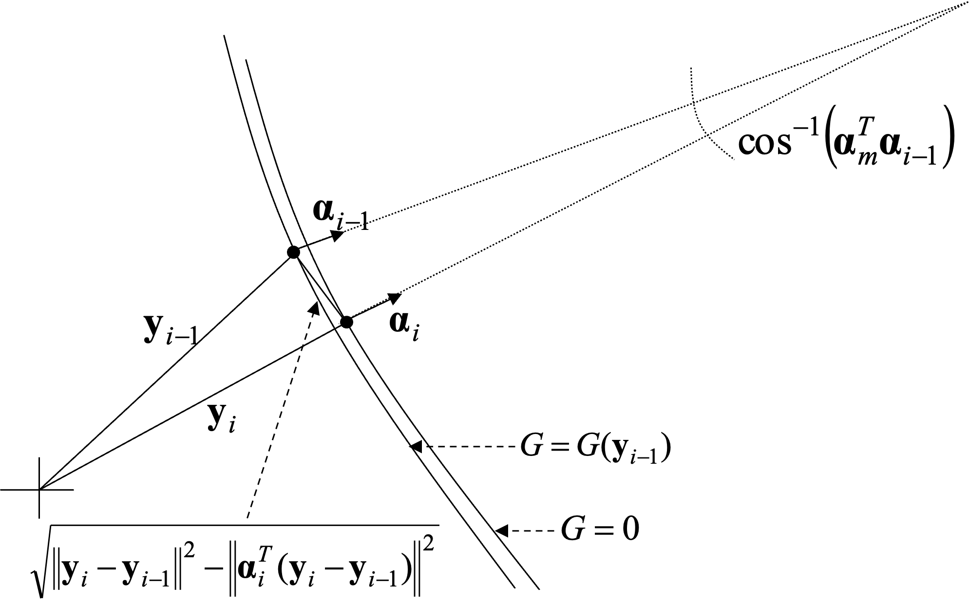
Interestingly, the iHLRF search approaches the design point such that the last points are approximately on the plane of the first principal curvature of the limit-state function in the \(\mathbf{y}\) space. That makes \(\kappa\) from Equation 6.17 valuable. However, as observed in the previous subsection, the limit-state function has as many curvatures as the number of random variables minus one. That prompted Der Kiureghian and Stefano (1991) to conduct new searches for the design point in spaces perpendicular to the plane of the curvatures found in previous searches. That is not done here, but the estimate of the first principal curvature is kept.
It is interesting to compare curvatures from Equation 6.17 with curvature calculated in the SORM algorithm in Listing 6.4:
print("First principal curvature from iHLRF design point search:")
print(f"{kappa:.5f}")
print('\n'"Curvatures from Hessian matrix:")
for i in range(len(curvatures)):
    print(f"{curvatures[i]:.5f}")
First principal curvature from iHLRF design point search:
0.05862
Curvatures from Hessian matrix:
0.04443
-0.03477
-0.02232
-0.00006We see there is reasonable but imperfect agreement between the curvature from Equation 6.17 and the first curvature from the algorithm Listing 6.4. Good agreement will be seen in examples later in this book. However, the failure probability estimate obtained by using only the single curvature from Equation 6.17 is less good. Oftentimes, higher-order curvatures matter. That is seen here, where beta and kappa calculated by the iHLRF algorithm earlier in this chapter are utilized and compared with the SORM result from the previous subsection:
print(f"FORM failure probability: {pfFORM:.5f}")
print(f"SORM failure probability: {pfSORM:.5f} (using all curvatures)")
newEstimate = pfFORM * 1.0 / np.sqrt(1.0 + beta * kappa)
print(f"SORM failure probability: {newEstimate:.5f} (using only first curvature)")
FORM failure probability: 0.02391
SORM failure probability: 0.02430 (using all curvatures)
SORM failure probability: 0.02263 (using only first curvature)