from Chapter10code import *11 Nonlinear SDOF Dynamics
In multi-DOF nonlinear dynamics it is easy to end up in an intellectual “paralysis by analysis.” That is because the number of modelling choices and available analysis results is large. For that reason, it is helpful to first study single-DOF problems. Essentially combining Equation 8.1 and Equation 10.1, the governing equilibrium equation, here enforced at time increment \(t_{n+1}\), is
\[ M\cdot \ddot{u}_{n+1} + C \cdot \dot{u}_{n+1} + \tilde{F}(u_{n+1}) = -M \cdot \ddot{u}_g(t_{n+1}) \tag{11.1}\]
where \(\tilde{F}=\) hysteretic spring force resisting displacement. That force is here modelled with the bilinear material model introduced in Chapter 8 and coded in Appendix A. In other words, \(\tilde{F}(u_{n+1})\) is the same as \(\sigma(\varepsilon_{n+1})\) in this chapter. Equation 10.15 is employed to express the damping coefficient in terms of the initial stiffness of that material:
\[ C = 2 \cdot \zeta \cdot \sqrt{K_o\cdot M} \tag{11.2}\]
The time-stepping scheme in Equation 10.39 is reused and adapted to the single-DOF case:
\[ \begin{aligned} \ddot{u}_{n+1} &= a_1 \cdot u_{n+1} + a_2 \cdot u_n + a_3 \cdot \dot{u}_n + a_4 \cdot \ddot{u}_n \\ \dot{u}_{n+1} &= a_5 \cdot u_{n+1} + a_6 \cdot u_n + a_7 \cdot \dot{u}_n + a_8 \cdot \ddot{u}_n \end{aligned} \tag{11.3}\]
The values for \(a_i\) given below Equation 10.39, for the Newmark beta method with constant average acceleration over each time interval, are employed in this chapter as well.
11.1 Newton-Raphson Method
Equation 11.1 and Equation 11.3 represent the temporally discretized problem addressed in this chapter. Written on residual form, the problem reads
\[ \begin{aligned} R &= M\cdot (a_1 \cdot u_{n+1} + a_2 \cdot u_n + a_3 \cdot \dot{u}_n + a_4 \cdot \ddot{u}_n) \\ &+ C \cdot (a_5 \cdot u_{n+1} + a_6 \cdot u_n + a_7 \cdot \dot{u}_n + a_8 \cdot \ddot{u}_n) \\ &+ \tilde{F}(u_{n+1}) + M \cdot \ddot{u}_g(t_{n+1}) = 0 \end{aligned} \tag{11.4}\]
Notice that \(u_{n+1}\) is the only unknown in that equation. The first-order Taylor approximation of the residual, omitting the \(n+1\) subscript for brevity, is similar to Equation 8.5 and Equation 8.6:
\[ R(u_{i+1}) \approx R(u_i) + \frac{\partial R}{\partial u_i} \cdot \Delta u_i \tag{11.5}\]
The index \(i+1\) means a new iteration compared to \(i\), but still at time increment \(t_{n+1}\). Setting the linearized residual equal to zero yields the following equation for \(\Delta u_i\), matching Equation 8.7:
\[ \Delta u_i = \frac{R(u_i)}{\left(\frac{\partial R}{\partial u_i} \right)} \tag{11.6}\]
The Newton-Raphson algorithm repeatedly solves Equation 11.6, steadily adding contributions to the trial displacement. For each new trial displacement, the state determination of the material model re-evaluates \(\tilde{F}\). The iterations continue until the residual is close to zero. As stated below Equation 8.7, the displacement accumulated within a time increment, not the entire analysis, is given to the hysteretic material model. The derivative of the residual in Equation 11.4 with respect to the displacement at iteration \(i\) at increment \(n+1\) is the effective dynamic stiffness:
\[ \frac{\partial R}{\partial u} = M\cdot a_1 + C \cdot a_5 + \frac{\partial \tilde{F}}{\partial u} \tag{11.7}\]
In the code presented after the sensitivity derivations, the stiffness \(K \equiv \frac{\partial \tilde{F}}{\partial u}\) is updated at every iteration in every increment.
11.2 First-order Sensitivities
The dependence of \(\tilde{F}\) on the variable \(x\), potentially explicitly but always implicitly via \(u_{n+1}\), is explained in Section 8.1.1. In the present context, this means the differentiation of the combined equations Equation 11.1 and Equation 11.3 reads
\[ \begin{aligned} &\phantom{+}\frac{\partial M}{\partial x} \left(a_1 \cdot u_{n+1} + a_2 \cdot u_n + a_3 \cdot \dot{u}_n + a_4 \cdot \ddot{u}_n \right) \\ &+ M \left(a_1 \cdot \frac{\partial u_{n+1}}{\partial x} + a_2 \cdot \frac{\partial u_n}{\partial x} + a_3 \cdot \frac{\partial \dot{u}_n}{\partial x} + a_4 \cdot \frac{\partial \ddot{u}_n}{\partial x} \right) \\ &+ \frac{\partial C}{\partial x} \left(a_5 \cdot u_{n+1} + a_6 \cdot u_n + a_7 \cdot \dot{u}_n + a_8 \cdot \ddot{u}_n \right) \\ &+ C \left(a_5 \cdot \frac{\partial u_{n+1}}{\partial x} + a_6 \cdot \frac{\partial u_n}{\partial x} + a_7 \cdot \frac{\partial \dot{u}_n}{\partial x} + a_8 \cdot \frac{\partial \ddot{u}_n}{\partial x} \right) \\ &+ K \cdot \frac{\partial u_{n+1}}{\partial x} - \left. \frac{\partial \tilde{F}}{\partial x} \right|_{u_{n+1} \: \mathrm{fixed}} = - \frac{\partial M}{\partial x} \cdot \ddot{u}_g(t_{n+1}) \end{aligned} \tag{11.8}\]
Sorting terms without the unknown, \(\frac{\partial u_{n+1}}{\partial x}\), to the right-hand side gives a linear equation for the first-order response sensitivity:
\[ \begin{aligned} \left(a_1 \cdot M + a_5 \cdot C + K \right) \frac{\partial u_{n+1}}{\partial x} &= - \frac{\partial M}{\partial x} \cdot \ddot{u}_g(t_{n+1}) \\ &- \frac{\partial M}{\partial x} \left(a_1 \cdot u_{n+1} + a_2 \cdot u_n + a_3 \cdot \dot{u}_n + a_4 \cdot \ddot{u}_n \right) \\ &- M \left(a_2 \cdot \frac{\partial u_n}{\partial x} + a_3 \cdot \frac{\partial \dot{u}_n}{\partial x} + a_4 \cdot \frac{\partial \ddot{u}_n}{\partial x} \right) \\ &- \frac{\partial C}{\partial x} \left(a_5 \cdot u_{n+1} + a_6 \cdot u_n + a_7 \cdot \dot{u}_n + a_8 \cdot \ddot{u}_n \right) \\ &- C \left(a_6 \cdot \frac{\partial u_n}{\partial x} + a_7 \cdot \frac{\partial \dot{u}_n}{\partial x} + a_8 \cdot \frac{\partial \ddot{u}_n}{\partial x} \right) \\ &- \left. \frac{\partial \tilde{F}}{\partial x} \right|_{u_{n+1} \: \mathrm{fixed}} \end{aligned} \tag{11.9}\]
As earlier in this book, we observe that \(u_{n+1}\) appears in that right-hand side, meaning that at each increment the displacement must be computed before its derivative is solved for. The derivative of the damping coefficient, needed in Equation 11.9, is obtained by differentiating Equation 11.2:
- \(\frac{\partial C}{\partial x} = 2 \cdot \sqrt{K_o \cdot M}\) if \(\zeta\) is the parameter that \(x\) represents
- \(\frac{\partial C}{\partial x} = \zeta \cdot \frac{K_o}{\sqrt{K_o \cdot M}}\) if \(M\) is the parameter that \(x\) represents
- \(\frac{\partial C}{\partial x} = \zeta \cdot \frac{M}{\sqrt{K_o \cdot M}}\) if \(K_o\) is the parameter that \(x\) represents
11.3 Second-order Sensitivities
The second differentiation of Equation 11.8 requires the second differentiation of \(\tilde{F}\). Labelling the variable in the first differentiation above by the symbol \(x_i\), the second differentiation is with respect to \(x_j\), giving five terms, matching those that appeared earlier in Equation 8.11:
\[ \begin{aligned} \frac{\partial^2 \tilde{F}}{\partial x_i \partial x_j} &=\frac{\partial K}{\partial u} \frac{\partial u_{n+1}}{\partial x_j} \frac{\partial u_{n+1}}{\partial x_i} + \left. \frac{\partial K}{\partial x_j} \right|_{u_{n+1} \: \mathrm{fixed}} \frac{\partial u_{n+1}}{\partial x_i} \\ &+ K \cdot \frac{\partial^2 u_{n+1}}{\partial x_i \partial x_j} + \left. \frac{\partial K}{\partial x_i} \right|_{u_{n+1} \: \mathrm{fixed}} \frac{\partial u_{n+1}}{\partial x_j} + \left. \frac{\partial^2 \tilde{F}}{\partial x_i \partial x_j} \right|_{u_{n+1} \: \mathrm{fixed}} \end{aligned} \tag{11.10}\]
Now including the mass and damping terms from Equation 11.1, second-order sensitivities are solved from
\[ \begin{aligned} &\phantom{+} \frac{\partial^2 M}{\partial x_i \partial x_j} \cdot \ddot{u}_{n+1} + \frac{\partial M}{\partial x_i} \frac{\partial \ddot{u}_{n+1}}{\partial x_j} + \frac{\partial M}{\partial x_j} \frac{\partial \ddot{u}_{n+1}}{\partial x_i} + M \cdot \frac{\partial^2 \ddot{u}_{n+1}}{\partial x_i \partial x_j} \\ &+ \frac{\partial^2 C}{\partial x_i \partial x_j} \cdot \dot{u}_{n+1} + \frac{\partial C}{\partial x_i} \frac{\partial \dot{u}_{n+1}}{\partial x_j} + \frac{\partial C}{\partial x_j} \frac{\partial \dot{u}_{n+1}}{\partial x_i} + C \cdot \frac{\partial^2 \dot{u}_{n+1}}{\partial x_i \partial x_j} \\ &+ \frac{\partial^2 \tilde{F}}{\partial x_i \partial x_j} = - \frac{\partial^2 M}{\partial x_i \partial x_j} \cdot \ddot{u}_g(t_{n+1}) \end{aligned} \tag{11.11}\]
where \(\frac{\partial^2 \tilde{F}}{\partial x_i \partial x_j}\) is given in Equation 11.10 and the derivatives of \(\ddot{u}_{n+1}\) and \(\dot{u}_{n+1}\) are obtained by differentiation of Equation 11.3. Carrying out that differentiation and sorting the terms without the unknown \(\frac{\partial^2 u_{n+1}}{\partial x_i \partial x_j}\) to the right-hand side gives the linear equation for the second-order response sensitivity:
\[ \begin{aligned} \left(a_1 \cdot M + a_5 \cdot C + K \right) \frac{\partial^2 u_{n+1}}{\partial x_i \partial x_j} &= \frac{\partial^2 M}{\partial x_i \partial x_j} \cdot \ddot{u}_{n+1} + \frac{\partial M}{\partial x_i} \frac{\partial \ddot{u}_{n+1}}{\partial x_j} + \frac{\partial M}{\partial x_j} \frac{\partial \ddot{u}_{n+1}}{\partial x_i} \\ &+ M \cdot \left(a_2 \cdot \frac{\partial^2 u_n}{\partial x_i \partial x_j} + a_3 \cdot \frac{\partial^2 \dot{u}_n}{\partial x_i \partial x_j} + a_4 \cdot \frac{\partial^2 \ddot{u}_n}{\partial x_i \partial x_j} \right) \\ &+ \frac{\partial^2 C}{\partial x_i \partial x_j} \cdot \dot{u}_{n+1} + \frac{\partial C}{\partial x_i} \frac{\partial \dot{u}_{n+1}}{\partial x_j} + \frac{\partial C}{\partial x_j} \frac{\partial \dot{u}_{n+1}}{\partial x_i} \\ &+ C \cdot \left(a_6 \cdot \frac{\partial^2 u_n}{\partial x_i \partial x_j} + a_7 \cdot \frac{\partial^2 \dot{u}_n}{\partial x_i \partial x_j} + a_8 \cdot \frac{\partial^2 \ddot{u}_n}{\partial x_i \partial x_j} \right) \\ &+ \frac{\partial^2 \tilde{F}}{\partial x_i \partial x_j} = - \frac{\partial^2 M}{\partial x_i \partial x_j} \cdot \ddot{u}_g(t_{n+1}) \end{aligned} \tag{11.12}\]
In addition to quantities from the previous increment, we observe that \(\frac{\partial u_{n+1}}{\partial x_i}\) and \(\frac{\partial u_{n+1}}{\partial x_j}\) appears in that right-hand side, meaning that at any given increment the first-order response derivative must be computed before the second-order derivative is solved for. In Equation 11.12, the second-order derivative of the mass is always zero: \(\frac{\partial^2 M}{\partial x_i \partial x_j}=0\). In contrast, several non-zero cases are possible in the second differentiation of Equation 11.2:
- \(\frac{\partial^2 C}{\partial x_i \partial x_j} = -\frac{M^2}{2\cdot \sqrt{K_o \cdot M}}\) if \(x_i=x_j=K_o\)
- \(\frac{\partial^2 C}{\partial x_i \partial x_j} = -\frac{K_o^2}{2\cdot \sqrt{K_o \cdot M}}\) if \(x_i=x_j=M\)
- \(\frac{\partial^2 C}{\partial x_i \partial x_j} = \frac{\zeta}{2\cdot \sqrt{K_o \cdot M}}\) if \(x_i=M\) and \(x_j=K_o\), or vice versa
- \(\frac{\partial^2 C}{\partial x_i \partial x_j} = \frac{K_o}{\sqrt{K_o \cdot M}}\) if \(x_i=M\) and \(x_j=\zeta\), or vice versa
- \(\frac{\partial^2 C}{\partial x_i \partial x_j} = \frac{M}{\sqrt{K_o \cdot M}}\) if \(x_i=K_o\) and \(x_j=\zeta\), or vice versa
11.4 Ground Motion Scaling
Little attention was given to the ground motion in the derivations above. However, it may be of interest to examine how the response changes if the ground motion is scaled. To that end, we rewrite the loading term in Equation 11.1 as
\[ F(t_n) = -M \cdot s \cdot \ddot{u}_g(t_n) \tag{11.13}\]
where \(s=\) scaling factor. However, the ground motion is not actually scaled in subsequent analyses. Rather, we determine the sensitivity with respect to a hypothetical scaling.
When \(s\) is the variable represented by \(x\) then we employ Equation 11.1 to add \(-M\cdot \ddot{u}_g(t_{n+1})\) to the right-hand side of Equation 11.9. Similarly, when \(s\) is the variable represented by \(x_i\) and \(M\) is the variable represented by \(x_j\), or vice versa, then \(-\ddot{u}_g(t_{n+1})\) is added to the right-hand side of Equation 11.12.
11.5 Analysis with Sensitivities
The algorithm presented below calculates first- and second-order response sensitivities alongside the nonlinear dynamic single-DOF response. Because the bilinear uniaxial material model is employed, the following six variables are candidates for sensitivity analysis: \(E\), \(f_y\), \(\alpha\), \(M\), \(\zeta\), and \(s\). The possible DDM request ‘GivenDerivative’ seen in the code below is employed in Chapter 13.
def nonlinearDynamicSDOFAnalysis(material, M, dampingRatio, groundMotion, DDMparameters=[], ddmRequest=0):

    # Ground motion
    t = groundMotion[0]
    dt = float(t[1] - t[0])
    groundAcceleration = groundMotion[1]
    numTimePoints = len(t)

    # Damping
    Kinitial = material.initialStiffness()
    C = 2 * np.sqrt(Kinitial * M) * dampingRatio

    # Initialization
    a1=4/dt**2; a2=-a1; a3=-4/dt; a4=-1; a5=2/dt; a6=-a5; a7=-1; a8=0
    u = np.zeros(3)
    displacementOld = 0.0
    velocityOld = 0.0
    accelerationOld = 0.0
    dnl = np.zeros(numTimePoints)
    uTrack = np.zeros(numTimePoints)
    vTrack = np.zeros(numTimePoints)
    aTrack = np.zeros(numTimePoints)

    numDDMparameters = len(DDMparameters)
    dudx = np.zeros((numDDMparameters, numTimePoints))
    dvdx = np.zeros((numDDMparameters, numTimePoints))
    dadx = np.zeros((numDDMparameters, numTimePoints))
    dudx2 = np.zeros((numDDMparameters, numDDMparameters, numTimePoints))
    if ddmRequest > 0 and numDDMparameters > 0:
        ddmDisplacementOld = np.zeros(numDDMparameters)
        ddmVelocityOld = np.zeros(numDDMparameters)
        ddmAccelerationOld = np.zeros(numDDMparameters)

    if ddmRequest > 1 and numDDMparameters > 0:
        triangularNumber = int(numDDMparameters * (numDDMparameters + 1) / 2)
        ddm2DisplacementOld = np.zeros(triangularNumber)
        ddm2VelocityOld = np.zeros(triangularNumber)
        ddm2AccelerationOld = np.zeros(triangularNumber)

    # Increments
    maxiter = 10
    tol = 1e-6
    for n in range(numTimePoints):

        # Iterations
        converged = False
        for ii in range(maxiter):
            F_tilde, K = material.stateDetermination(u)
            F = -M * groundAcceleration[n]
            R = -F
            R += F_tilde
            massFactor = a1*u[0] + a2*displacementOld + a3*velocityOld + a4*accelerationOld
            R += M * massFactor
            dampingFactor = a5*u[0] + a6*displacementOld + a7*velocityOld + a8*accelerationOld
            R += C * dampingFactor
            # Check convergence
            if np.abs(R) < tol:
                converged = True
                break
            Keffective = K + a1 * M + a5 * C
            u[2] = -R / Keffective
            u[0] = u[0] + u[2]
            u[1] = u[1] + u[2]
        if not converged:
            print('\n'"No convergence with residual", R, ">", tol, "in", maxiter, "iterations for time step", n)
            import sys
            sys.exit()

        velocityNew = a5 * u[0] + a6 * displacementOld + a7 * velocityOld + a8 * accelerationOld
        accelerationNew = a1 * u[0] + a2 * displacementOld + a3 * velocityOld + a4 * accelerationOld
        dnl[n] = K/Kinitial
        uTrack[n] = u[0]
        vTrack[n] = velocityNew
        aTrack[n] = accelerationNew + groundAcceleration[n]

        # First-order sensitivities
        if ddmRequest > 0 and numDDMparameters > 0:
            F_tilde, K = material.stateDetermination(u)
            Keffective = K + a1 * M + a5 * C
            if ddmRequest > 1:
                dMdxStorage = []
                dCdxStorage = []
                dKdxStorage = []
                dudxStorage = []
                dvdxStorage = []
                dadxStorage = []
            for ddmIndex in range(len(DDMparameters)):
                ddmRHS = 0.0
                dM = 0.0
                dC = 0.0
                if DDMparameters[ddmIndex][0] == 'Material':
                    dF_tilde, dK, dKmdum = material.stateDerivative(u, DDMparameters[ddmIndex][1], ddmIndex, True)
                    ddmRHS -= dF_tilde
                    if DDMparameters[ddmIndex][1] == 'E':
                        dC = M / np.sqrt(M * Kinitial) * dampingRatio
                else:
                    dF_tilde, dK, dKmdum = material.stateDerivative(u, 'Void', ddmIndex, False)
                    ddmRHS -= dF_tilde
                    if DDMparameters[ddmIndex][0] == 'Mass':
                        ddmRHS -= groundAcceleration[n]
                        dM = 1
                        dC = Kinitial / np.sqrt(Kinitial * M) * dampingRatio
                    elif DDMparameters[ddmIndex][0] == 'GroundMotion' and DDMparameters[ddmIndex][1] == 'Scaling':
                        ddmRHS -= M * groundAcceleration[n]
                    elif DDMparameters[ddmIndex][0] == 'GroundMotion' and DDMparameters[ddmIndex][1] == 'GivenDerivative':
                        gmDerivative = groundMotion[DDMparameters[ddmIndex][2]+1][n]
                        ddmRHS = ddmRHS - M * gmDerivative
                    elif DDMparameters[ddmIndex][0] == 'Damping':
                        dC = 2 * np.sqrt(Kinitial * M)

                ddmRHS -= M * (a2 * ddmDisplacementOld[ddmIndex] + a3 * ddmVelocityOld[ddmIndex] + a4 * ddmAccelerationOld[ddmIndex])
                ddmRHS -= C * (a6 * ddmDisplacementOld[ddmIndex] + a7 * ddmVelocityOld[ddmIndex] + a8 * ddmAccelerationOld[ddmIndex])
                ddmRHS -= dM * (a1 * u[0] + a2 * displacementOld + a3 * velocityOld + a4 * accelerationOld)
                ddmRHS -= dC * (a5 * u[0] + a6 * displacementOld + a7 * velocityOld + a8 * accelerationOld)
                ddmDisplacementNew = ddmRHS / Keffective
                ddmAccelerationNew = a1 * ddmDisplacementNew + a2 * ddmDisplacementOld[ddmIndex] + a3 * ddmVelocityOld[ddmIndex] + a4 * ddmAccelerationOld[ddmIndex]
                ddmVelocityNew = a5 * ddmDisplacementNew + a6 * ddmDisplacementOld[ddmIndex] + a7 * ddmVelocityOld[ddmIndex] + a8 * ddmAccelerationOld[ddmIndex]
                if ddmRequest > 1:
                    dMdxStorage.append(dM)
                    dCdxStorage.append(dC)
                    dKdxStorage.append(dK)
                    dudxStorage.append(ddmDisplacementNew)
                    dvdxStorage.append(ddmVelocityNew)
                    dadxStorage.append(ddmAccelerationNew)
                ddmDisplacementOld[ddmIndex] = ddmDisplacementNew
                ddmVelocityOld[ddmIndex] = ddmVelocityNew
                ddmAccelerationOld[ddmIndex] = ddmAccelerationNew
                ddmu = ddmDisplacementNew
                dudx[ddmIndex, n] = ddmu
                dvdx[ddmIndex, n] = ddmVelocityNew
                dadx[ddmIndex, n] = ddmAccelerationNew
                if DDMparameters[ddmIndex][0] == 'Material':
                    material.commitSensitivity(u, ddmu, DDMparameters[ddmIndex][1], ddmIndex, True)
                else:
                    material.commitSensitivity(u, ddmu, 'Void', ddmIndex, False)

            # Second-order sensitivities
            if ddmRequest > 1:
                secondOrderIndex = -1
                for ddmIndex2 in range(len(DDMparameters)):
                    for ddmIndex1 in range(ddmIndex2+1):
                        secondOrderRHS = 0.0
                        secondOrderIndex += 1
                        ddmIsHere1 = False
                        ddmIsHere2 = False
                        parameter1 = DDMparameters[ddmIndex1][0]
                        parameter2 = DDMparameters[ddmIndex2][0]
                        if parameter1 == 'Material':
                            ddmIsHere1 = True
                            parameter1 = DDMparameters[ddmIndex1][1]
                        if parameter2 == 'Material':
                            ddmIsHere2 = True
                            parameter2 = DDMparameters[ddmIndex2][1]
                        ddsigma, ddK = material.stateSecondDerivative(u, secondOrderIndex, parameter1, ddmIndex1, ddmIsHere1, parameter2, ddmIndex2, ddmIsHere2)
                        secondOrderRHS -= ddsigma
                        if (parameter1 == 'GroundMotion' and DDMparameters[ddmIndex1][1] == 'Scaling' and parameter2 == 'Mass') or (parameter2 == 'GroundMotion' and DDMparameters[ddmIndex2][1] == 'Scaling' and parameter1 == 'Mass'):
                            secondOrderRHS -= groundAcceleration[n]
                        secondOrderRHS = secondOrderRHS - dKdxStorage[ddmIndex1] * dudxStorage[ddmIndex2]
                        parenthesis = dKmdum * dudxStorage[ddmIndex2] + dKdxStorage[ddmIndex2]
                        secondOrderRHS = secondOrderRHS - parenthesis * dudxStorage[ddmIndex1]
                        secondOrderRHS = secondOrderRHS - dMdxStorage[ddmIndex1] * dadxStorage[ddmIndex2]
                        secondOrderRHS = secondOrderRHS - dMdxStorage[ddmIndex2] * dadxStorage[ddmIndex1]
                        secondOrderRHS = secondOrderRHS - M * (a2 * ddm2DisplacementOld[secondOrderIndex] + a3 * ddm2VelocityOld[secondOrderIndex] + a4 * ddm2AccelerationOld[secondOrderIndex])
                        ddC = 0.0
                        if parameter1 == 'E' and parameter2 == 'E':
                            ddC = -0.5 / (Kinitial*M)**(1.5) * M**2 * dampingRatio
                        elif parameter1 == 'Mass' and parameter2 == 'Mass':
                            ddC = -0.5 / (Kinitial*M)**(1.5) * Kinitial**2 * dampingRatio
                        elif (parameter1 == 'E' and parameter2 == 'Mass') or (parameter1 == 'Mass' and parameter2 == 'E'):
                            ddC = dampingRatio / (2 * np.sqrt(Kinitial*M))
                        elif (parameter1 == 'Damping' and parameter2 == 'Mass') or (parameter1 == 'Mass' and parameter2 == 'Damping'):
                            ddC = Kinitial / np.sqrt(Kinitial * M)
                        elif (parameter1 == 'Damping' and parameter2 == 'E') or (parameter1 == 'E' and parameter2 == 'Damping'):
                            ddC = M / np.sqrt(Kinitial * M)
                        secondOrderRHS = secondOrderRHS - ddC * velocityNew
                        secondOrderRHS = secondOrderRHS - dCdxStorage[ddmIndex1] * dvdxStorage[ddmIndex2]
                        secondOrderRHS = secondOrderRHS - dCdxStorage[ddmIndex2] * dvdxStorage[ddmIndex1]
                        secondOrderRHS = secondOrderRHS - C * (a6 * ddm2DisplacementOld[secondOrderIndex] + a7 * ddm2VelocityOld[secondOrderIndex] + a8 * ddm2AccelerationOld[secondOrderIndex])
                        ddm2DisplacementNew = secondOrderRHS / Keffective
                        ddm2AccelerationNew = a1 * ddm2DisplacementNew + a2 * ddm2DisplacementOld[secondOrderIndex] + a3 * ddm2VelocityOld[secondOrderIndex] + a4 * ddm2AccelerationOld[secondOrderIndex]
                        ddm2VelocityNew = a5 * ddm2DisplacementNew + a6 * ddm2DisplacementOld[secondOrderIndex] + a7 * ddm2VelocityOld[secondOrderIndex] + a8 * ddm2AccelerationOld[secondOrderIndex]
                        dudx2[ddmIndex1, ddmIndex2, n] = ddm2DisplacementNew
                        dudx2[ddmIndex2, ddmIndex1, n] = ddm2DisplacementNew
                        ddm2DisplacementOld[secondOrderIndex] = ddm2DisplacementNew
                        ddm2AccelerationOld[secondOrderIndex] = ddm2AccelerationNew
                        ddm2VelocityOld[secondOrderIndex] = ddm2VelocityNew
                        material.commitSecondSensitivity(u, dudxStorage[ddmIndex1], dudxStorage[ddmIndex2], ddm2DisplacementNew, secondOrderIndex, parameter1, ddmIndex1, ddmIsHere1, parameter2, ddmIndex2, ddmIsHere2)
        material.commit()
        displacementOld = u[0]
        velocityOld = velocityNew
        accelerationOld = accelerationNew
        u[1] = 0.0

    return t, uTrack, vTrack, aTrack, dudx, dvdx, dadx, dudx2, dnl
A few remarks are made about that algorithm:
- The material model has a function that returns its initial stiffness; notice that \(K_o \equiv E\) in the derivations above.
- The total acceleration response is stored for reasons described in Section 10.3
- The functions
stateDerivative,stateSecondDerivative,commitSensitivity, andcommitSecondSensitivityare called even when the variable is not a material parameter; this is an important detail in sensitivity analysis with hysteretic material models
The nine returned quantities are:
tis the array that contains the time axis, \(\mathbf{t}\)uTrackis the relative displacement response at all time incrementsvTrackis the relative velocity response at all time incrementsaTrackis the total acceleration response, including the ground acceleration, at all time incrementsdudxis a matrix of first-order displacement sensitivities, \(\frac{\partial u[i, n]}{\partial x_i}\), where \(i\) is the index of the variable and \(n\) is the index of the time incrementdvdxis a matrix of first-order velocity sensitivities, \(\frac{\partial \dot{u}[i, n]}{\partial x_i}\), where \(i\) is the index of the variable and \(n\) is the index of the time incrementdadxis a matrix of first-order acceleration sensitivities, \(\frac{\partial \ddot{u}[i, n]}{\partial x_i}\), where \(i\) is the index of the variable and \(n\) is the index of the time incrementdudx2is a tensor of second-order displacement sensitivities, \(\frac{\partial^2 u[i, j, n]}{\partial x_i \partial x_j}\), where \(i\) is the index of the first variable, \(j\) is the index of the second variable, and \(n\) is the index of the time incrementdnlis the “degree of nonlinearity,” i.e., the ratio of the current stiffness to the initial stiffness at all time increments
In the analysis run below, the variable uy is the yield displacement and the mass, \(M\), is calculated from a given target natural period of vibration:
Tn = 0.5      # seconds
E = 1e4       # N/m
alpha = 0.05  # Dimensionless
uy = 0.03     # m
fy = E * uy   # N
material = bilinearMaterial(['Bilinear', E, fy, alpha])
M = (Tn/2/np.pi)**2 * E
dampingRatio = 0.05
dt = 0.02
gmMatrix = readGroundMotion("ElCentro.txt", dt)
DDMparameters = [['Material', 'E'],
                 ['Material', 'fy'],
                 ['Material', 'alpha'],
                 ['Mass'],
                 ['Damping'],
                 ['GroundMotion', 'Scaling']]
t, u, v, a, dudx, dvdx, dadx, dudx2, dnl = nonlinearDynamicSDOFAnalysis(material, M, dampingRatio, gmMatrix, DDMparameters, 2)
plt.figure()
for i in range(1, len(u)):
    if dnl[i] < 1:
        plt.plot([t[i-1], t[i]], [u[i-1], u[i]], 'r-', linewidth=1.0)
    else:
        plt.plot([t[i-1], t[i]], [u[i-1], u[i]], 'k-', linewidth=1.0)
plt.xlabel("Time [sec.]")
plt.ylabel("Displacement [m]")
plt.grid(True)
plt.show()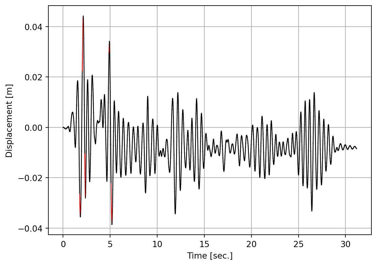
The red line in that plot identifies increments with yielding, i.e., with stiffness less than the initial stiffness. We see that some yielding takes place early in the time series, when the El Centro ground motion has the highest acceleration values.
Next, response sensitivities are examined with a 10% uniform coefficient of variation on all variables to enable a comparison of the individual sensitivities:
plt.figure()
plt.plot(t, dudx[0]*0.1*E, 'b-', linewidth=1.0, label='$\\frac{\\partial u}{\\partial E}$')
plt.plot(t, dudx[1]*0.1*fy, 'r-', linewidth=1.0, label='$\\frac{\\partial u}{\\partial f_y}$')
plt.plot(t, dudx[2]*0.1*alpha, 'g-', linewidth=1.0, label='$\\frac{\\partial u}{\\partial \\alpha}$')
plt.plot(t, dudx[3]*0.1*M, 'm-', linewidth=1.0, label='$\\frac{\\partial u}{\\partial M}$')
plt.plot(t, dudx[4]*0.1*dampingRatio, 'c-', linewidth=1.0, label='$\\frac{\\partial u}{\\partial \\zeta}$')
plt.plot(t, dudx[5]*0.1, 'y-', linewidth=1.0, label='$\\frac{\\partial u}{\\partial s}$')
plt.xlabel("Time [sec.]")
plt.legend(loc='upper right')
plt.grid(True)
plt.show()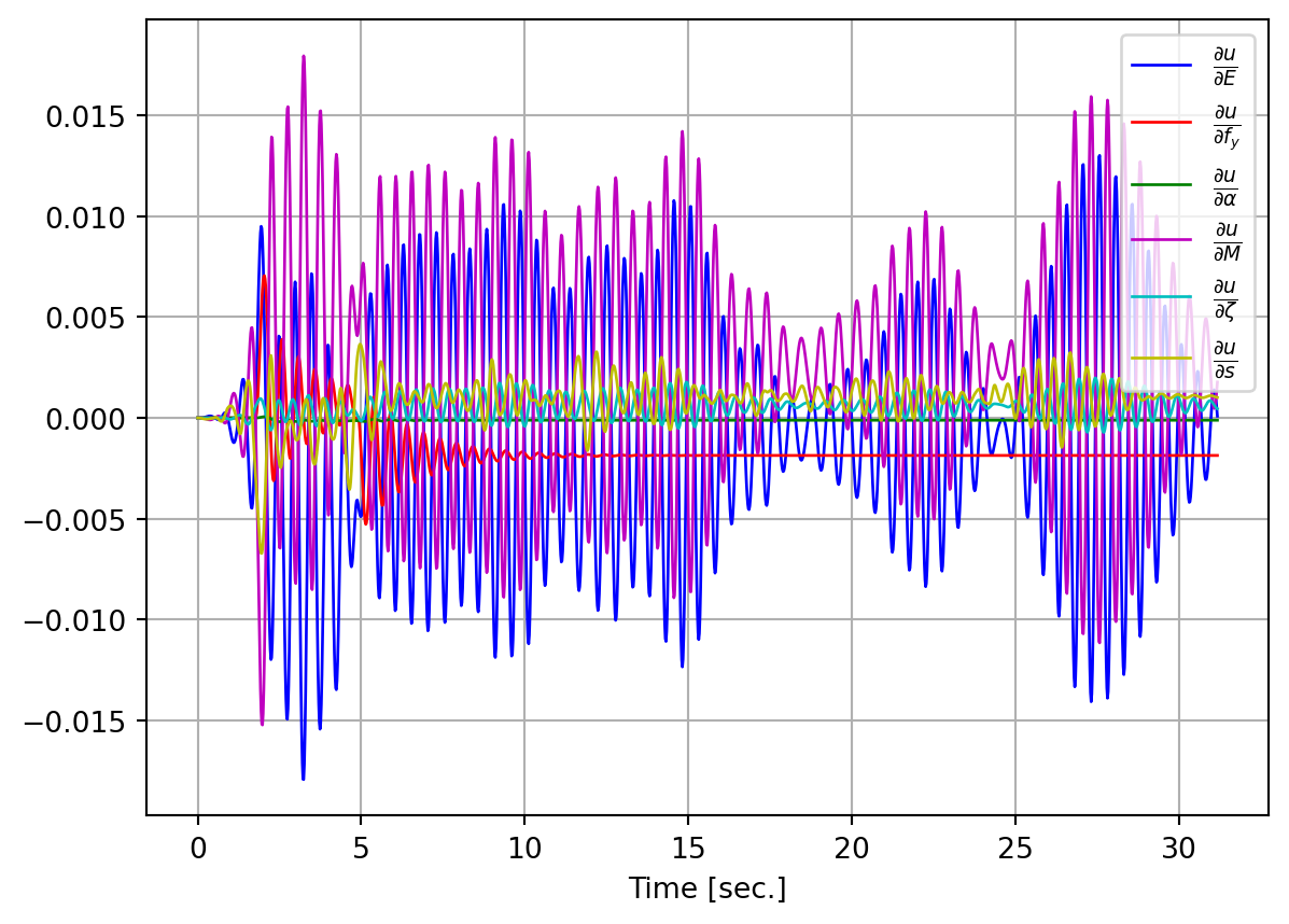
As was noted in the previous chapter, plotting sensitivities along the full time axis can make the results hard to read. Zooming in on a time window and adding the displacement to the plot gives:
timeWindow = range(int(0.12*len(t)), int(0.18*len(t)))
plt.figure()
for i in timeWindow:
    if dnl[i] < 1:
        plt.plot([t[i-1], t[i]], [u[i-1], u[i]], 'r-', linewidth=1.0)
    else:
        plt.plot([t[i-1], t[i]], [u[i-1], u[i]], 'k-', linewidth=1.0)
plt.plot(t[timeWindow], dudx[0, timeWindow]*0.1*E, 'b-', linewidth=1.0, label='$\\frac{\\partial u}{\\partial E}$')
plt.plot(t[timeWindow], dudx[1, timeWindow]*0.1*fy, 'r-', linewidth=1.0, label='$\\frac{\\partial u}{\\partial f_y}$')
plt.plot(t[timeWindow], dudx[2, timeWindow]*0.1*alpha, 'g-', linewidth=1.0, label='$\\frac{\\partial u}{\\partial \\alpha}$')
plt.plot(t[timeWindow], dudx[3, timeWindow]*0.1*M, 'm-', linewidth=1.0, label='$\\frac{\\partial u}{\\partial M}$')
plt.plot(t[timeWindow], dudx[4, timeWindow]*0.1*dampingRatio, 'c-', linewidth=1.0, label='$\\frac{\\partial u}{\\partial \\zeta}$')
plt.plot(t[timeWindow], dudx[5, timeWindow]*0.1, 'y-', linewidth=1.0, label='$\\frac{\\partial u}{\\partial s}$')
plt.xlabel("Time [sec.]")
plt.legend(loc='upper right')
plt.grid(True)
plt.show()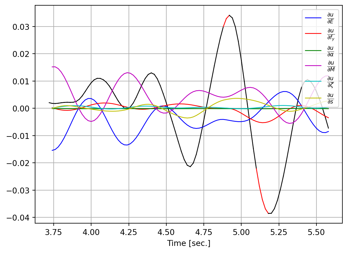
That plot shows that the stiffness and mass sensitivities are no longer sure to be near zero when the response peaks, as it was in the linear analysis in the previous chapter. Furthermore, the sensitivity with respect to those two variables remains high, now in the company of the scaling factor. As in the previous chapter, the sensitivity to damping appears to be low.