from Chapter2code import *3 Linear Static Analysis
In a habit established in the first chapter, Python functions from the previous chapter are here imported. Note that this import statement, issued in every chapter, is nested. The code imported here from the previous chapter issues an import statement for the code in the chapter before that, and so on:
The governing equilibrium equations for linear static structural analysis are given in Section 1.6 followed by baseline equations for first- and second-order response sensitivity analysis. Utilizing the computational infrastructure presented in Chapter 2, the objective now is to solve Equation 1.4, Equation 1.8, and Equation 1.10 for \(\mathbf{u}\), \(\frac{\partial \mathbf{u}}{\partial x}\) and \(\frac{\partial^2 \mathbf{u}}{\partial x_i \partial x_j}\), respectively.
In solving those tasks, the orchestrating algorithm communicates with the elements of the structural model. In turn, in the nonlinear analysis later in this book, the elements communicate with its cross-section objects, which in turn communicate with its material models. With an eye to that more advanced analysis, the notation and protocols for the communication is first established.
3.1 Force Vector Notation
The communication between the elements and the structural analysis algorithm is aided by the following notation:
- Internal forces that resist displacements:
- \(\mathbf{Ku}\) in linear analysis
- \(\tilde{\mathbf{F}}(\mathbf{u})\) in nonlinear analysis
- Force vector at the structural level from applied loads:
- \(\mathbf{F}=\overset{\backprime}{\mathbf{F}}-\bar{\mathbf{F}}\)
- \(\overset{\backprime}{\mathbf{F}}\) are point loads applied directly along DOFs
- \(\bar{\mathbf{F}}\) are fixed-end forces from loads along elements
- \(\mathbf{F}=\overset{\backprime}{\mathbf{F}}-\bar{\mathbf{F}}\)
- Force vector at the element level from given displacements and element loads:
- \(\mathbf{F}=\mathbf{Ku} + \bar{\mathbf{F}}\) in linear analysis
- \(\mathbf{F}=\tilde{\mathbf{F}}(\mathbf{u}) + \bar{\mathbf{F}}\) in nonlinear analysis
The very last item in that list, applicable to nonlinear analysis, has a bearing on the naming of symbols in the linear analysis code presented in this chapter. That is because elements developed for nonlinear analysis return those two contributions, i.e., \(\mathbf{F}=\tilde{\mathbf{F}}(\mathbf{u}) + \bar{\mathbf{F}}\), in one vector when asked for its internal forces for a given displacement.
Therefore, in order to utilize linear elastic elements in nonlinear analysis, conformity in the communication protocol is needed. That is why the linear elastic element developed in this chapter returns the force vector \(\mathbf{F}=\mathbf{Ku} + \bar{\mathbf{F}}\). As a reminder of that fact, the returned force vector and its derivatives in sensitivity analysis are given the label Both in the code.
With the notation established above, we must still dig a little deeper to fully undestand the code presented in this chapter. First, notice that in linear analysis the displacements \(\mathbf{u}\) are zero when the call is made to the elements to deliver its stiffness matrix and force vector. That is why, in linear analysis, it is indeed only the element forces \(\bar{\mathbf{F}}\) that are returned from the element.
That said, the aforementioned label Both is still warranted in this book for linear analysis. That is because, in first-order sensitivity analysis, the elements must return the terms \(\frac{\partial \bar{\mathbf{F}}}{\partial x}\) and \(\frac{\partial \mathbf{K}}{\partial x}\mathbf{u}\) for the right-hand side of the governing system of equations in Equation 1.8. As will be seen later, this means returning \(\frac{\partial \bar{\mathbf{F}}}{\partial x}\) and \(\frac{\partial \tilde{\mathbf{F}}}{\partial x}\) in nonlinear analysis, with the latter then being a derivative for fixed displacements. In nonlinear analysis, both those terms are returned in one vector, with the stiffness matrix addressing other needs.
Because the nonlinear elements do that, the linear elastic element presented below does the same. We notice that this is the derivative of the vector labelled Both above, i.e., \(\frac{\partial \mathbf{K}}{\partial x}\mathbf{u} + \frac{\partial \bar{\mathbf{F}}}{\partial x}\). Moreover, that sum corresponds exactly to the negative of the right-hand side of Equation 1.8, because \(\bar{\mathbf{F}}\) enters the final load vector \(\mathbf{F}\) with opposite sign. This is why the label Both remains appropriate in sensitivity analysis, where the returned vector does have two contributions.
In the same way, for second-order response sensitivities, the elements return both \(\frac{\partial^2 \mathbf{F}}{\partial x_i \partial x_j}\) and \(\frac{\partial^2 \mathbf{K}}{\partial x_i \partial x_j} \mathbf{u}\) in one vector labelled Both, for the governing equations in Equation 1.10. Again, this matches the return of two terms in one vector in nonlinear analysis. It is also the reason why the elements never actually return \(\frac{\partial^2 \mathbf{K}}{\partial x_i \partial x_j}\). Stay tuned for increased understanding of the details of response sensitivity analysis as the reading progresses.
3.2 Format for Requesting Sensitivities
When we get to the point that the DDM has been implemented, we need to issue requests to tell the analysis which responses and which response sensitivities are sought. For now, here are a few arbitrary examples to help understand the code presented next, with more examples coming thereafter:
['Element', 'E', [1, 2, 3]gives \(\frac{\partial u}{\partial x}\) for \(x\) representing the modulus of elasticity in Elements 1, 2, and 3['Element', 'q', [1]]gives \(\frac{\partial u}{\partial x}\) for \(x\) representing a distributed load on Element 1['Nodal load', 2, 1]gives \(\frac{\partial u}{\partial x}\) for \(x\) representing a point load at Node 2 along its DOF 1
3.3 Linear Elastic Frame Element
The constructor of the linear elastic frame element class, Element 5, was established in Chapter 2. It is now time to populate the class with member functions that provide its stiffness matrix, etc. In matrix structural analysis, which is the computational implementation of the stiffness method, transformation matrices serve an important role in that regard. That is because the element sees several “DOF configurations” in the process that establishes the stiffness matrix and force vector ultimately given to the structural analysis.
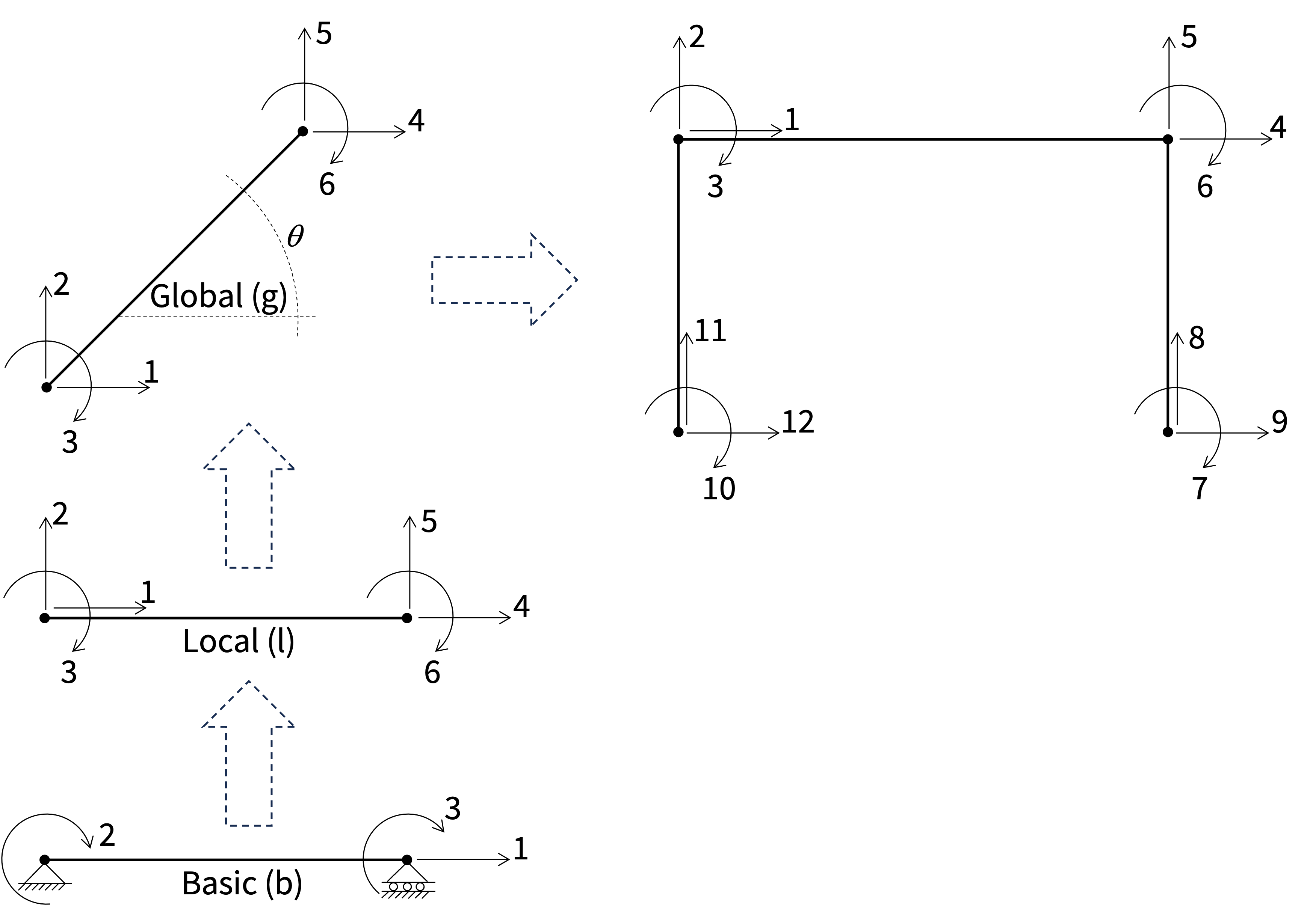
Figure 3.1 provides an overview of the process, identifying the Basic, Local, and Global element configurations:
- Basic: Statically determinate element with sufficient DOFs to describe any deformation, but no rigid body motion
- Local: Adding DOFs to enable rigid body motion
- Global: Accounts for the orientation of the element in the global coordinate system that the structural model occupies
3.3.1 Transformation Matrices
A hallmark of displacement-based analysis methods is that transformation matrices connect the DOFs in separate configurations. The transformation matrices relevant for Figure 3.1 are \(\mathbf{T}_{bl}\) and \(\mathbf{T}_{lg}\). Subscripts reflect the configurations they connect. That means \(\mathbf{T}_{bl}\) connects the Basic and Local configurations. The equation that defines \(\mathbf{T}_{bl}\) is \(\mathbf{u}_{b}=\mathbf{T}_{bl}\mathbf{u}_{l}\). By setting the DOFs \(\mathbf{u}_{l}\) equal to unity, one at a time, the columns of \(\mathbf{T}_{bl}\) are established, one by one. Specifically, each column is the \(\mathbf{u}_{b}\) vector corresponding to the aforementioned unit DOF value. It is helpful to draw displaced shapes when doing that work, giving the result
\[ \mathbf{T}_{bl} = \begin{bmatrix} -1 & 0 & 0 & 1 & 0 & 0 \\ 0 & -\frac{1}{L} & 1 & 0 & \frac{1}{L} & 0 \\ 0 & -\frac{1}{L} & 0 & 0 & \frac{1}{L} & 1 \end{bmatrix} \tag{3.1}\]
\(\mathbf{T}_{lg}\) is established in a similar manner, with the defining relationship \(\mathbf{u}_{l}=\mathbf{T}_{lg}\mathbf{u}_{g}\):
\[ \mathbf{T}_{lg} = \begin{bmatrix} \cos(\theta) & \sin(\theta) & 0 & 0 & 0 & 0 \\ -\sin(\theta) & \cos(\theta) & 0 & 0 & 0 & 0 \\ 0 & 0 & 1 & 0 & 0 & 0 \\ 0 & 0 & 0 & \cos(\theta) & \sin(\theta) & 0 \\ 0 & 0 & 0 & -\sin(\theta) & \cos(\theta) & 0 \\ 0 & 0 & 0 & 0 & 0 & 1 \end{bmatrix} \tag{3.2}\]
\(\theta\) is defined in Figure 3.1. For efficiency, the matrix product \(\mathbf{T}_{bg}=\mathbf{T}_{bl}\mathbf{T}_{lg}\) is carried out, once and for all, before implementation in Python: \[ \mathbf{T}_{bg} = \begin{bmatrix} -c_x & -c_y & 0 & c_x & c_y & 0 \\ \frac{c_y}{L} & -\frac{c_x}{L} & 1 & -\frac{c_y}{L} & \frac{c_x}{L} & 0 \\ \frac{c_y}{L} & -\frac{c_x}{L} & 0 & -\frac{c_y}{L} & \frac{c_x}{L} & 1 \\ \end{bmatrix} \tag{3.3}\]
Here, the notation \(c_x \equiv \frac{\Delta x}{L}\) and \(c_y \equiv \frac{\Delta y}{L}\) is introduced for the “direction cosines” of the element. With the help of Figure 3.2 we find that \(c_x = \cos(\theta)\) and \(c_x = \sin(\theta)\).
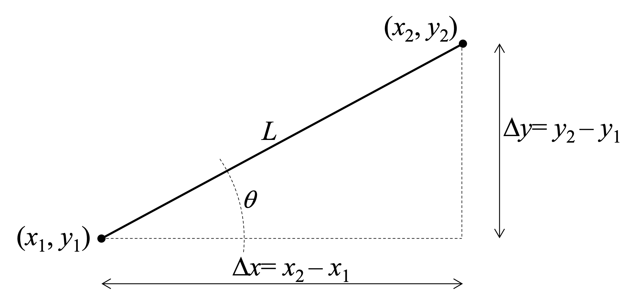
To avoid recalculating the components of \(\mathbf{T}_{bg}\) in the response sensitivity analysis, it is implemented in the initialize() function shown below. That function is called at the start of any structural analysis, and it would be prudent to use that function to also check that the element length is non-zero, for example. In the implementation of Equation 3.2 shown below, it is the input xyz that contains the coordinates of the two nodes of the element, facilitating the calculation of the direction cosines:
class element5(element5):
    def initialize(self, xyz):
        dx = xyz[1,:] - xyz[0,:]
        L = np.sqrt(dx.dot(dx))
        dx = dx/L
        cos = dx[0]
        sin = dx[1]
        cosL = cos/L
        sinL = sin/L
        self.Tbg = np.array([[-cos,  -sin,  0,  cos,  sin,  0],
                             [ sinL, -cosL, 1, -sinL, cosL, 0],
                             [ sinL, -cosL, 0, -sinL, cosL, 1]])
        self.L = L
        self.cos = cos
        self.sin = sin
3.3.2 Force Vector & Stiffness Matrix
The transformation matrices derived above enter a bigger picture. It is a picture that appears in many places in structural analysis, from simple beam theory to advanced finite element methods. One name that may be given to the picture is the boundary value problem of structural analysis. It has three ingredients:
- Equilibrium
- Material law
- Kinematic compatibility
A fourth ingredient is boundary conditions, which are case-specific. Figure 3.3 shows the ingredients of the boundary value problem that involves the DOF configurations already introduced. Kinematic compatibility relationships, described above as defining the transformation matrices, appear on the right-hand side of Figure 3.3.
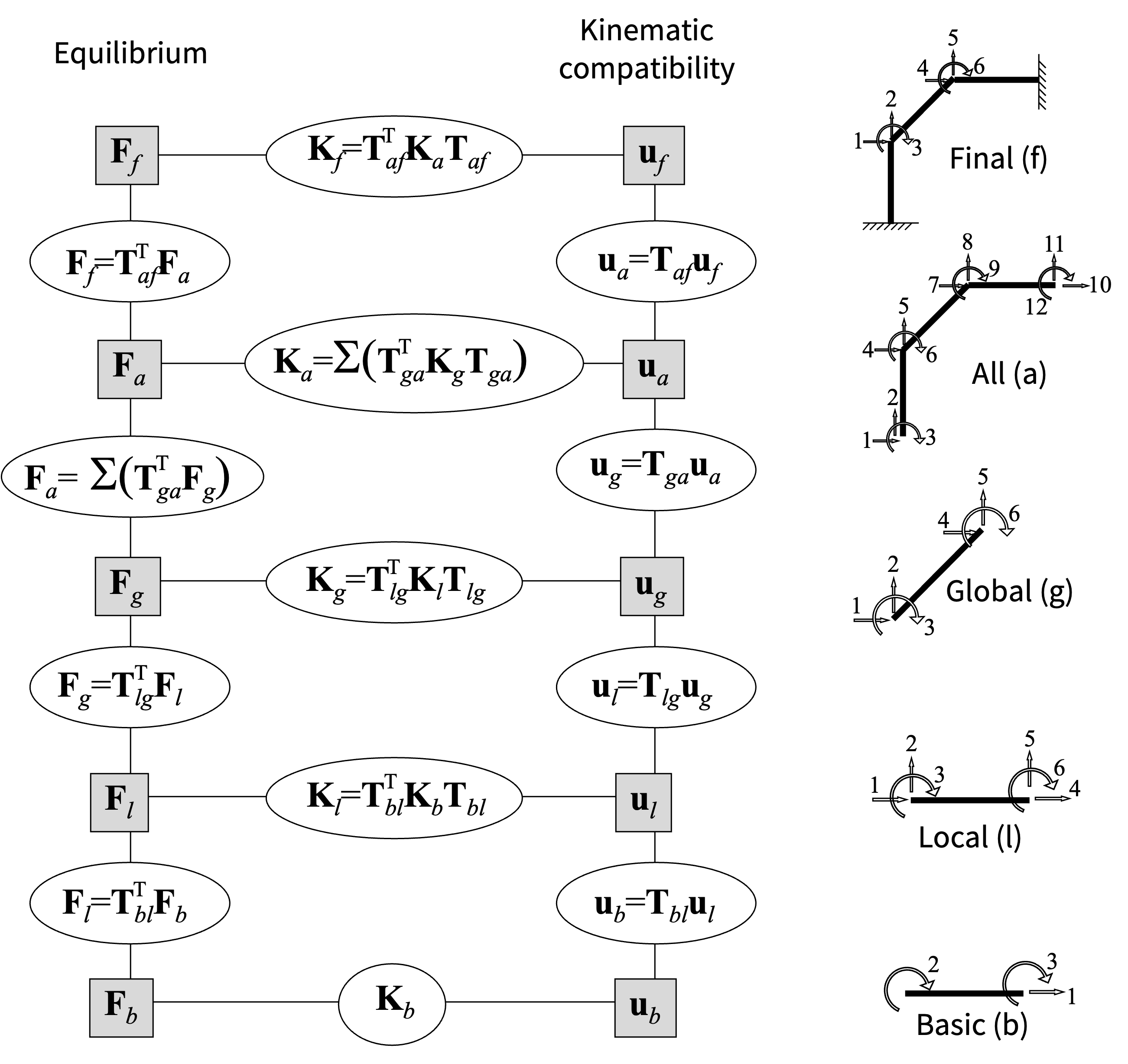
An objective now is to derive the equilibrium relationships that appear in the left-hand side of Figure 3.3. Consider the Basic and Local configurations, where we seek the relationship between \(\mathbf{F}_b\) and \(\mathbf{F}_l\). The starting point is the principle of virtual displacements on residual form, i.e., with a zero right-hand side:
\[ \mathbf{F}_l^{\top} \delta \mathbf{u}_l - \mathbf{F}_b^{\top} \delta \mathbf{u}_b = 0 \tag{3.4}\]
Substitution of the kinematic compatibility equation \(\mathbf{u}_{b}=\mathbf{T}_{bl}\mathbf{u}_{l}\) into Equation 3.4 gives
\[ \mathbf{F}_l^{\top} \delta \mathbf{u}_l - \mathbf{F}_b^{\top} \mathbf{T}_{bl} \delta \mathbf{u}_{l} =\left( \mathbf{F}_l^{\top} - \mathbf{F}_b^{\top} \mathbf{T}_{bl} \right) \delta \mathbf{u}_{l} = 0 \tag{3.5}\]
Because \(\delta \mathbf{u}_{l}\) are arbitrary virtual displacements, only needing to satisfy the displacement boundary conditions, the parenthesis in Equation 3.5 must be zero, which means that
\[ \mathbf{F}_l^{\top} - \mathbf{F}_b^{\top} \mathbf{T}_{bl} = 0 \tag{3.6}\]
Taking the transpose of Equation 3.6 and moving one term to the right-hand side yields
\[ \mathbf{F}_l = \mathbf{T}_{bl}^{\top} \mathbf{F}_b \tag{3.7}\]
That relationship is observed in the lower-right corner of Figure 3.3. It says that equilibrium employs the same transformation matrix as was established on the kinematic compatibility side. However, in contrast to compatibility, the transformation matrix appears transposed in equilibrium. In fact, the following two complementary statements can be made:
- Kinematic compatibility is expressed as displacements in the DOF configuration below being equal to the transformation matrix times the displacements in the configuration above
- Equilibrium is expressed as forces in the DOF configuration above being equal to the transformation matrix transposed times the forces in the configuration below
The next goal is to determine the stiffness matrix in a configuration “above” knowing the stiffness matrix in the configuration immediately “below.” Still considering the step from Basic to Local, the following three ingredients form the starting point:
- Equilibrium: \(\mathbf{F}_l = \mathbf{T}_{bl}^{\top} \mathbf{F}_b\)
- Material law: \(\mathbf{F}_b = \mathbf{K}_{b} \mathbf{u}_b\)
- Kinematic compatibility: \(\mathbf{u}_{b}=\mathbf{T}_{bl}\mathbf{u}_{l}\)
Substitution if Item 3 into Item 2, and substituting the restult into Item 1 yields
\[ \mathbf{F}_l = \underbrace{\mathbf{T}_{bl}^{\top} \mathbf{K}_{b} \mathbf{T}_{bl}}_{\mathbf{K}_l} \mathbf{u}_{l} \tag{3.8}\]
where the stiffness matrix in the configuration above is identified. This completes the proofs of the relationships given in Figure 3.3. In the element calculations shown next, the stiffness matrix in the Global configuration is calculated from the stiffness matrix in the Basic configuration, using the following Python statement:
Kg = (np.transpose(self.Tbg).dot(Kb)).dot(self.Tbg)
In passing, it is noted that a neat and efficient alternative is offered by Einstein’s summation convention in index notation, explained in the next chapter:
Kg = np.einsum('ji,jk,kl->il', Tbg, Kb, Tbg)
3.3.3 State Determination
Although Element 5 is a linear elastic frame element, it must have features that allow it to be used in nonlinear analysis. That is why the member function that provides the element stiffness matrix is called stateDetermination(). State determination in nonlinear analysis means determining stiffness and internal forces for a given trial displacement. In nonlinear analysis, addressed in later chapters, the displacements are given incrementally to the elements, allowing for hysteretic material behaviour. This matter simplifies for linear elastic elements, where the stiffness is always the same, and the internal forces are simply stiffness times displacement. Four arguments appear in the signature of the state determination code below:
selfis the mandatory first argument for member functions of a class in Pythonxyzcoordinates of the two nodes attached to the elementugcontains \(\mathbf{u}_g\); however, for the purpose of nonlinear analysis, covered later in this book, three \(\mathbf{u}_g\) vectors are given to the element, making it a matrix (only the total displacement is employed in this element)theLambdais the load factor used in nonlinear analysis
The second half of the state determination below is about including distributed element load, \(q\), in the force vector that is returned together with the stiffness matrix:
class element5(element5):
    def stateDetermination(self, xyz, ug, theLambda):
        EI = self.E * self.I
        EA = self.E * self.A
        L = self.L
        self.Kb = np.array([[EA/L, 0.0,    0.0],
                            [0.0,  4*EI/L, 2*EI/L],
                            [0.0,  2*EI/L, 4*EI/L]])
        Kg = (np.transpose(self.Tbg).dot(self.Kb)).dot(self.Tbg)
        q = theLambda * self.q
        FEM = q * L**2 / 12.0
        FbBar = [0.0, -FEM, FEM]
        shearBar = q*L/2.0
        FbBoth = (self.Kb.dot(self.Tbg)).dot(ug[:,0]) + FbBar
        FgBoth = (np.transpose(self.Tbg)).dot(FbBoth) + np.array([-self.sin*shearBar, self.cos*shearBar, 0.0, -self.sin*shearBar, self.cos*shearBar, 0.0])
        return FgBoth, Kg
It is here restated that the displacements, \(\mathbf{u}_g\), given to the element are zero when the state determination is called in linear analysis. That means the vector \(\mathbf{F}_{\mathrm{Both}}=\mathbf{Ku} + \bar{\mathbf{F}}\) that is returned above simply contains the fixed-end forces from \(q\) in this case.
3.3.4 First-order Sensitivities
The input variables to the linear elastic frame element are \(E\), \(A\), \(I\), and \(q\), defined early in Chapter 2. The job of the element, in terms of first-order sensitivity analysis, is to prepare for the possible order to return the derivative of the force vector and the stiffness matrix with respect to those input variables. In other words, we seek the ingredients of the two terms on the right-hand side of Equation 1.8.
When the call goes out to all elements that ingredients are needed for sensitivity calculations, two pieces of information follows the order given to each element:
ddmParameteris a string with the name of the variable, such as"E","A", or"I"ddmIsHereis a boolean flag that isTrueif the variable resides in the element being called, otherwiseFalse
Those items explain statements like if ddmParameter == 'E' and ddmIsHere in the member function for first-order sensitivity analysis shown below. The arguments self, xyz, ug, theLambda are explained before Listing 3.2, while ddmIndex and dKflag are only used in nonlinear analysis, addressed later in this book. To that end, the calculation of first-order sensitivities in the linear element is done as follows:
class element5(element5):
    def stateDerivative(self, xyz, ug, theLambda, ddmParameter, ddmIndex=0, ddmIsHere=False, dkflag='none'):
        if ddmParameter == 'E' and ddmIsHere:
            dEI = self.I
            dEA = self.A
        elif ddmParameter == 'A' and ddmIsHere:
            dEI = 0.0
            dEA = self.E
        elif ddmParameter == 'I' and ddmIsHere:
            dEI = self.E
            dEA = 0.0
        else:
            dEI = 0.0
            dEA = 0.0
        L = self.L
        dKb = np.array([[dEA/L, 0.0,    0.0],
                        [0.0,  4*dEI/L, 2*dEI/L],
                        [0.0,  2*dEI/L, 4*dEI/L]])
        dKg = (np.transpose(self.Tbg).dot(dKb)).dot(self.Tbg)
        dFb = (dKb.dot(self.Tbg)).dot(ug[:,0])
        dFgBoth = (np.transpose(self.Tbg)).dot(dFb)
        if ddmParameter == 'q':
            q = theLambda
            dFEM = q * L**2 / 12.0
            dFb_bar = [0.0, -dFEM, dFEM]
            dShearBar = q*L/2.0
            dFgBoth = (np.transpose(self.Tbg)).dot(dFb_bar) + np.array([-self.sin*dShearBar, self.cos*dShearBar, 0.0, -self.sin*dShearBar, self.cos*dShearBar, 0.0])
        return dFgBoth, dKg, 0
The 0 returned above relates to the dKflag input, which is relevant in nonlinear dynamic analyses, where a non-zero value is required for certain damping models. Because the derivative of the stiffness matrix is used to calculate dFgBoth it is not needed in the orchestrating analysis algorithm. Still, dKg is returned, because it is needed in the calculation of second-order sensitivities.
3.3.5 Second-order Sensitivities
Equation 1.10 is the linear system of equations that governs the calculation of the second-order response sensitivities, \(\frac{\partial^2 \mathbf{u}}{\partial x_i \partial x_j}\). Disregarding quantities already available, the right-hand side of that equation requires the calculation of \(\frac{\partial^2 \mathbf{F}}{\partial x_i \partial x_j}\) and \(\frac{\partial^2 \mathbf{K}}{\partial x_i \partial x_j}\). This task is addressed by differentiating the algorithm in Listing 3.3. As commented on earlier in this chapter, we observe that \(\frac{\partial^2 \mathbf{K}}{\partial x_i \partial x_j}\) is employed within this function; that quantity is therefore not returned:
class element5(element5):
    def stateSecondDerivative(self, xyz, ug, theLambda, secondOrderIndex, ddmParameter1, ddmIndex1, ddmIsHere1, ddmParameter2, ddmIndex2, ddmIsHere2):
        ddEI = 0
        ddEA = 0
        if ddmParameter1 == 'E' and ddmIsHere1:
            if ddmParameter2 == 'I' and ddmIsHere2:
                ddEI = 1
            if ddmParameter2 == 'A' and ddmIsHere2:
                ddEA = 1
        elif ddmParameter1 == 'A' and ddmIsHere1:
            if ddmParameter2 == 'E' and ddmIsHere2:
                ddEA = 1
        elif ddmParameter1 == 'I' and ddmIsHere1:
            if ddmParameter2 == 'E' and ddmIsHere2:
                ddEI = 1
        L = self.L
        ddKb = np.array([[ddEA/L, 0.0,    0.0],
                        [0.0,  4*ddEI/L, 2*ddEI/L],
                        [0.0,  2*ddEI/L, 4*ddEI/L]])
        ddFbBoth = (ddKb.dot(self.Tbg)).dot(ug[:,0])
        ddFgBoth = (np.transpose(self.Tbg)).dot(ddFbBoth)
        return ddFgBoth
3.3.6 Adding Element to Model
In Chapter 2, a rudimentary member function of the structural model, named createElements() was created. In the present chapter, the member functions of Element 5 has been defined. Therefore, it is time to redefine the createElements() function, giving it the ability to create linear elastic frame elements:
class model(model):
    def createElements(self):
        nelem = len(self.ELEMENTS)
        ellist = []
        for i in range(nelem):
            eltyp = self.ELEMENTS[i][0]
            if eltyp == 5:
                E = self.ELEMENTS[i][1]
                A = self.ELEMENTS[i][2]
                I = self.ELEMENTS[i][3]
                q = self.ELEMENTS[i][4]
                el = element5(E, A, I, q, i+1)
            ellist.append(el)
        return ellist
3.4 Response Algorithms & Frame Example
The portal frame input is created in the previous chapter by the function defined in Listing 2.1. The advantage of that approach, allowing that model to be used repeatedly, carries over to a more detailed specification the input variables. Both for sensitivity analysis, and for subsequent reliability analyses, it is helpful to keep the following specifications within a function:
def linearFrameVariableSpecs():
    E = 200e9         # N/m^2
    A = 18774e-6      # m^2
    I = 462016882e-12 # m^4
    q = 20e3          # N/m
    F = 50e3          # N
    covE = 0.1
    covA = 0.05
    covI = 0.05
    covq = 0.2
    covF = 0.2
    means = [     E,      A,      I,      q,      F]
    stdvs = [covE*E, covA*A, covI*I, covq*q, covF*F]
    distributions = ['Lognormal', 'Lognormal', 'Lognormal', 'Lognormal', 'Lognormal']
    correlation = [[4, 5, 0.75]]
    trackNode = 2
    trackDOF = 1
    DDMs = [['Element', 'E', [1, 2, 3]],
            ['Element', 'A', [1, 2, 3]],
            ['Element', 'I', [1, 2, 3]],
            ['Element', 'q', [1]],
            ['Nodal load', 2, 1]]

    return means, stdvs, distributions, correlation, trackNode, trackDOF, DDMs
The coefficients of variation, means, standard deviations, and distributions given in Listing 3.6 are not relevant in this chapter. The material and cross-section values given above correspond to a W14x99 = SI-W360X147 wide-flange steel cross-section. The DDMs array says that we seek \(\frac{\partial u}{\partial E}\), \(\frac{\partial u}{\partial A}\), \(\frac{\partial u}{\partial I}\), \(\frac{\partial u}{\partial q}\), and \(\frac{\partial u}{\partial F}\), where \(u=\) horizontal displacement at the upper left corner of the frame, i.e., DOF 1 at Node 2, and \(F=\) horizontal load at the same location. Notice the [1, 2, 3] input in the DDMs array, meaning that the derivatives, such as \(\frac{\partial u}{\partial E}\), is for \(E\) as a single variable in all three elements of the portal frame. The second-order response sensitivity analysis implemented below calculates exact double- and cross-derivatives between those variables.
3.4.1 Response Analysis
An algorithm to calculate the structural response, but not response sensitivities, is implemented below. Adopting notation from the previous chapter, quantities that address “all” structural DOFs, regardless of whether they are free or fixed, are labelled a. Similarly, those that cover the “free” DOFs of the structure are labelled f:
def linearStaticResponse(model, trackNode, trackDOF):
    ndof, ntot, Fa, M, elemlist = model.getData()
    free = range(ndof)
    nelem = len(elemlist)
    dof = model.DOF[trackNode - 1, trackDOF - 1]
    FaBoth = np.zeros(ntot)
    ua = np.zeros((ntot,3))
    Ka = np.zeros((ntot, ntot))
    for eleNum in range(nelem):
        id, xyz, ug = model.localize(eleNum, ua)
        element = elemlist[eleNum]
        element.initialize(xyz)
        FgBoth, Kg = element.stateDetermination(xyz, ug, 1.0)
        Ka[np.ix_(id, id)] = Ka[np.ix_(id,id)] + Kg
        FaBoth[id] = FaBoth[id] + FgBoth
    Kf = Ka[np.ix_(free, free)]
    Ff = Fa[free] - FaBoth[free]
    ua[free, 0] = np.linalg.solve(Kf, Ff)
    return ua[dof, 0]
That function is tested on the portal frame established above, giving the following displacement response:
means, stdvs, void, void, trackNode, trackDOF, DDMs = linearFrameVariableSpecs()
input = createLinearFrameInput(*means)
structuralModel = model(input)
u = linearStaticResponse(structuralModel, trackNode, trackDOF)
print(f"Displacement: u={u:.4f}")
Displacement: u=0.01653.4.2 First-order Sensitivities
In linear static analysis we take advantage of the adjoint method, explained in Chapter 1, to calculate response sensitivities repeatedly, for many variables, simply by a dot product. Regardless of how many variables \(\mathbf{x}\) contains, the system of equations in Equation 1.15 is solved only once. However, as described in Chapter 1, the adjoint method can be applied either to calculate first-order sensitivities or second-order sensitivities, not both. This is why the function that calculates only first-order sensitivities, by the adjoint method, is here provided without any second-order sensitivity calculations:
def linearStaticFirstOrder(model, trackNode, trackDOF, DDMparameters):
    ndof, ntot, Fa, M, elemlist = model.getData()
    free = range(ndof)
    nelem = len(elemlist)
    dof = model.DOF[trackNode - 1, trackDOF - 1]
    FaBoth = np.zeros(ntot)
    ua = np.zeros((ntot,3))
    Ka = np.zeros((ntot, ntot))
    for eleNum in range(nelem):
        id, xyz, ug = model.localize(eleNum, ua)
        element = elemlist[eleNum]
        element.initialize(xyz)
        FgBoth, Kg = element.stateDetermination(xyz, ug, 1.0)
        Ka[np.ix_(id, id)] = Ka[np.ix_(id,id)] + Kg
        FaBoth[id] = FaBoth[id] + FgBoth
    Kf = Ka[np.ix_(free, free)]
    Ff = Fa[free] - FaBoth[free]
    numDDMparameters = len(DDMparameters)
    dudx = np.zeros(numDDMparameters)
    s = np.zeros(ntot)
    s[dof] = 1
    soln = np.linalg.solve(Kf, np.c_[Ff, s[free]])
    ua[free, 0] = soln[:, 0]
    lamda = soln[:, 1]
    for ddmIndex in range(numDDMparameters):
        ddmRHSa = np.zeros(ntot)
        if DDMparameters[ddmIndex][0] == 'Element':
            for eleNum in DDMparameters[ddmIndex][2]:
                id, xyz, ug = model.localize(eleNum-1, ua)
                element = elemlist[eleNum-1]
                dFgBoth, void, void = element.stateDerivative(xyz, ug, 1.0, DDMparameters[ddmIndex][1], 0, True)
                ddmRHSa[id] = ddmRHSa[id] - dFgBoth
        elif DDMparameters[ddmIndex][0] == 'Nodal load':
            loadIndex = model.DOF[DDMparameters[ddmIndex][1]-1, DDMparameters[ddmIndex][2]-1]
            ddmRHSa[loadIndex] = np.sign(Fa[loadIndex])
        dudx[ddmIndex] = np.dot(lamda, ddmRHSa[free])
    return ua[dof, 0], dudx
For the five variables in Listing 3.6 that algorithm provides five first-order response sensitivities, forming what is called the gradient vector:
\[ \nabla u \equiv \frac{\partial u}{\partial \mathbf{x}} = \begin{Bmatrix} \frac{\partial u}{\partial E} \\ \frac{\partial u}{\partial A} \\ \frac{\partial u}{\partial I} \\ \frac{\partial u}{\partial q} \\ \frac{\partial u}{\partial F} \end{Bmatrix} \tag{3.9}\]
Application of the function in Listing 3.8 to the portal frame gives the following gradient vector:
names = ['E', 'A', 'I', 'q', 'F']
u, dudx = linearStaticFirstOrder(structuralModel, trackNode, trackDOF, DDMs)
print(f"Displacement: u={u:.4f}")
for i in range(len(DDMs)):
    print(f"dud{names[i]} = {dudx[i]:.3e}")
Displacement: u=0.0165
dudE = -8.256e-14
dudA = -4.315e-03
dudI = -3.556e+01
dudq = 4.212e-07
dudF = 1.618e-073.4.3 Second-order Sensitivities
In Section 1.8 it was stressed that the adjoint method cannot be applied consecutively to calculate first-order sensitivities and then second-order sensitivities. That is why, if second-order response sensitivities are sought, we must shift the use of the adjoint method to those calculations. The following algorithm calculates the response, then first-order sensitivities without the adjoint method, and then the second-order sensitivities with the adjoint method:
def linearStaticSecondOrder(model, trackNode, trackDOF, DDMparameters):
    ndof, ntot, Fa, M, elemlist = model.getData()
    free = range(ndof)
    nelem = len(elemlist)
    dof = model.DOF[trackNode - 1, trackDOF - 1]
    FaBoth = np.zeros(ntot)
    ua = np.zeros((ntot,3))
    Ka = np.zeros((ntot, ntot))
    for eleNum in range(nelem):
        id, xyz, ug = model.localize(eleNum, ua)
        element = elemlist[eleNum]
        element.initialize(xyz)
        FgBoth, Kg = element.stateDetermination(xyz, ug, 1.0)
        Ka[np.ix_(id, id)] = Ka[np.ix_(id,id)] + Kg
        FaBoth[id] = FaBoth[id] + FgBoth
    Kf = Ka[np.ix_(free, free)]
    Ff = Fa[free] - FaBoth[free]
    numDDMparameters = len(DDMparameters)
    dudx = np.zeros((numDDMparameters, ntot))
    dudx2 = np.zeros((numDDMparameters, numDDMparameters))
    s = np.zeros(ntot)
    s[dof] = 1
    soln = np.linalg.solve(Kf, np.c_[Ff, s[free]])
    ua[free, 0] = soln[:, 0]
    lamda = soln[:, 1]
    dKaStorage = []
    for ddmIndex in range(numDDMparameters):
        ddmRHSa = np.zeros(ntot)
        dKa = np.zeros((ntot, ntot))
        if DDMparameters[ddmIndex][0] == 'Element':
            for eleNum in DDMparameters[ddmIndex][2]:
                id, xyz, ug = model.localize(eleNum-1, ua)
                element = elemlist[eleNum-1]
                dFgBoth, dKg, dKgdug = element.stateDerivative(xyz, ug, 1.0, DDMparameters[ddmIndex][1], 0, True)
                ddmRHSa[id] = ddmRHSa[id] - dFgBoth
                dKa[np.ix_(id, id)] = dKa[np.ix_(id,id)] + dKg
        elif DDMparameters[ddmIndex][0] == 'Nodal load':
            loadIndex = model.DOF[DDMparameters[ddmIndex][1]-1, DDMparameters[ddmIndex][2]-1]
            ddmRHSa[loadIndex] = np.sign(Fa[loadIndex])
        dudx[ddmIndex, free] = np.linalg.solve(Kf, ddmRHSa[free])
        dKaStorage.append(dKa)
    for ddmIndex2 in range(numDDMparameters):
        for ddmIndex1 in range(ddmIndex2+1):
            ddm2RHSa = np.zeros(ntot)
            if DDMparameters[ddmIndex1][0] == 'Element' and DDMparameters[ddmIndex2][0] == 'Element':
                ddmIsHere1 = np.full(nelem, False)
                for eleNum in DDMparameters[ddmIndex1][2]:
                    ddmIsHere1[eleNum-1] = True
                ddmIsHere2 = np.full(nelem, False)
                for eleNum in DDMparameters[ddmIndex2][2]:
                    ddmIsHere2[eleNum-1] = True
                for eleNum in range(nelem):
                    id, xyz, ug = model.localize(eleNum, ua)
                    element = elemlist[eleNum]
                    ddFgBoth = element.stateSecondDerivative(xyz, ug, 1.0, 0, DDMparameters[ddmIndex1][1], ddmIndex1, ddmIsHere1[eleNum], DDMparameters[ddmIndex2][1], ddmIndex2, ddmIsHere2[eleNum])
                    ddm2RHSa[id] = ddm2RHSa[id] + ddFgBoth
            ddm2RHSa = ddm2RHSa - dKaStorage[ddmIndex1].dot(dudx[ddmIndex2, :]) - dKaStorage[ddmIndex2].dot(dudx[ddmIndex1, :])
            dudx2[ddmIndex1, ddmIndex2] = np.dot(lamda, ddm2RHSa[free])
            dudx2[ddmIndex2, ddmIndex1] = np.dot(lamda, ddm2RHSa[free])
    return ua[dof, 0], dudx[:, dof], dudx2
In the algorithm shown above, notice how \(\frac{\partial \mathbf{u}}{\partial x}\) vectors and \(\frac{\partial \mathbf{K}}{\partial x}\) matrices are stored from the first-order calculations for the parenthesis in Equation 1.17. For the five variables in Listing 3.6 the function given above provides second-order sensitivities that can be arranged into what is called the Hessian matrix:
\[ \mathbf{H} \equiv \frac{\partial^2 u}{\partial x_i \partial x_j} = \begin{bmatrix} \frac{\partial^2 u}{\partial E^2} & \frac{\partial^2 u}{\partial E \partial A} & \frac{\partial^2 u}{\partial E \partial I} & \frac{\partial^2 u}{\partial E \partial q} & \frac{\partial^2 u}{\partial E \partial F} \\ \frac{\partial^2 u}{\partial A \partial E} & \frac{\partial^2 u}{\partial A^2} & \frac{\partial^2 u}{\partial A \partial I} & \frac{\partial^2 u}{\partial A \partial q} & \frac{\partial^2 u}{\partial A \partial F} \\ \frac{\partial^2 u}{\partial I \partial E} & \frac{\partial^2 u}{\partial I \partial A} & \frac{\partial^2 u}{\partial I^2} & \frac{\partial^2 u}{\partial I \partial q} & \frac{\partial^2 u}{\partial I \partial F} \\ \frac{\partial^2 u}{\partial q \partial E} & \frac{\partial^2 u}{\partial q \partial A} & \frac{\partial^2 u}{\partial q \partial I} & \frac{\partial^2 u}{\partial q^2} & \frac{\partial^2 u}{\partial q \partial F} \\ \frac{\partial^2 u}{\partial F \partial E} & \frac{\partial^2 u}{\partial F \partial A} & \frac{\partial^2 u}{\partial F \partial I} & \frac{\partial^2 u}{\partial F \partial q} & \frac{\partial^2 u}{\partial F^2} \end{bmatrix} \tag{3.10}\]
Application of the function in Listing 3.9 to the portal frame gives the following result:
u, dudx, dudx2 = linearStaticSecondOrder(structuralModel, trackNode, trackDOF, DDMs)
print(f"Displacement: u={u:.4f}")
for i in range(len(DDMs)):
    print(f"dud{names[i]} = {dudx[i]:.3e}")
print("Hessian:")
for i in range(len(DDMs)):
    for j in range(len(DDMs)):
        print(f"{dudx2[i][j]:11.3e}", end="")
    print(' ')
Displacement: u=0.0165
dudE = -8.256e-14
dudA = -4.315e-03
dudI = -3.556e+01
dudq = 4.212e-07
dudF = 1.618e-07
Hessian:
8.256e-25 6.473e-14 5.335e-10 -2.106e-18 -8.088e-19
6.473e-14 4.585e-01 4.615e-02 -1.042e-07 -4.463e-08
5.335e-10 4.615e-02 1.539e+05 -9.074e-04 -3.483e-04
-2.106e-18 -1.042e-07 -9.074e-04 0.000e+00 0.000e+00
-8.088e-19 -4.463e-08 -3.483e-04 0.000e+00 0.000e+00 The exact response sensitivities, calculated in an efficient manner above, are verified by approximate and more computationally costly finite different calculations in Chapter 14.
3.4.4 Importance Ranking
The results presented above enter into the analyses conducted in the next several chapters. They also answer the question “How sensitive is the response to a change in the input variables.” However, it is not possible to use first-order response sensitivities to tell which input variable is most important. In other words, it is not possible to use the results provided above to tell which variable the response is most sensitive to.
That is because the components of the gradient vector in Equation 3.9 have different units. To that end, we need the concept of importance vectors to complement the sensitivity vectors. The simplest importance vector is \(\left| \frac{\partial u}{\partial x_i}\cdot \sigma_i \right|\), where \(\sigma_i\) is the standard deviation of \(x_i\). That formula is casually stated to be the change in the response for a “reasonable” change in each parameter value, with all components of the importance vector having the unit of the displacement. Utilizing the coefficients of variation given in Listing 3.6, the five variables of the portal frame have the following relative importance:
importanceVector = dudx*stdvs
sortedVector = np.flip(np.argsort(np.abs(importanceVector)))
rank = 1
for i in sortedVector:
    print(f"Ranked {rank} is {names[i]} with dudx*stdv = {importanceVector[i]:.3e}"); rank+=1
Ranked 1 is q with dudx*stdv = 1.685e-03
Ranked 2 is E with dudx*stdv = -1.651e-03
Ranked 3 is F with dudx*stdv = 1.618e-03
Ranked 4 is I with dudx*stdv = -8.215e-04
Ranked 5 is A with dudx*stdv = -4.051e-06That output shows that the load \(q\) is the most important variable for the roof displacement of the portal frame. The least important variable by far is \(A\). The ranking is based on the absolute value of \(\frac{\partial u}{\partial x_i}\cdot \sigma_i\) but the sign is included in the printout. The sign tells us whether the variable is acting as a “resistance” or a “load” variable. The negative signs in the output above says that \(E\), \(I\), and \(A\) are resistance variables, meaning that their increase would cause a decrease in \(u\). Conversely, the output reasonably suggests that \(q\) and \(F\) are load variables, meaning that their increase would cause an increase in the displacement response.