from Chapter13code import *14 Finite Difference Checks
The DDM, introduced in Chapter 1 and implemented throughout this book, provides exact and efficiently calculated response sensitivities. It comes at a one-time cost of implementation of analytical derivatives alongside the ordinary response calculations. It is important that those implementations are checked and debugged if errors are detected. To check the DDM implementations, the finite difference approach is helpful. Although it only gives approximate response sensitivites, and requires one new structural analysis for every variable in \(\mathbf{x}\), it serves as a good debugging tool. First-order sensitivities by the finite difference approach are calculated by
\[ \frac{\partial u}{\partial x} \approx \frac{u(x+\Delta x) - u(x))}{\Delta x} \tag{14.1}\]
where \(u(x+\Delta x)\) is the response from a new structural analysis with the parameter \(x\) perturbed by the amount \(\Delta x\). Similarly, second-order response sensitivities from finite difference are calculated by
\[ \frac{\partial^2 u}{\partial x_i \partial x_j} \approx \frac{\frac{\partial u(x_j+\Delta x_j)}{\partial x_i} - \frac{\partial u(x_j)}{\partial x_i}}{\Delta x_j} \tag{14.2}\]
with verified first-order derivatives provided by the structural analysis algorithm. The finite difference approach in Equation 14.1 and Equation 14.2 is employed to verify the implementations offered in previous chapters.
The perturbation, \(\Delta x\), is expressed via the following perturbed variable value:
\[ x_{\textrm{perturbed}} = x_{\textrm{original}} \cdot (1+\textrm{perturbationFraction}) \tag{14.3}\]
The following choice is made in this chapter:
perturbationFraction = 1e-614.1 Linear Static
The linear elastic portal frame analyzed in the early chapters of this book is here re-created, and plotted as a reminder of its shape:
means, stdvs, void, void, trackNode, trackDOF, DDMs = linearFrameVariableSpecs()
input = createLinearFrameInput(*means)
structuralModel = model(input)
structuralModel.plotModel()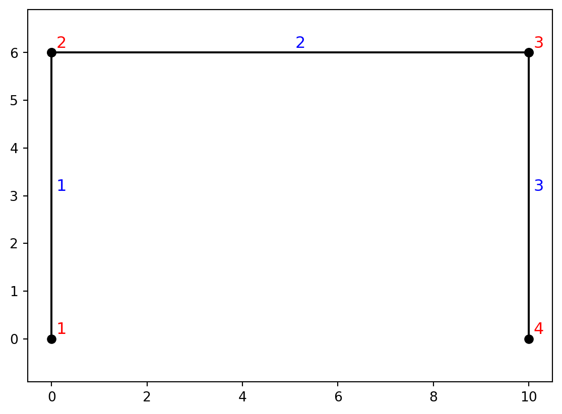
The objective now is to check the sensitivity calculations by finite difference. Sensitivities were calculated in two functions for linear static analysis, and they are both run here:
u, dudxA = linearStaticFirstOrder(structuralModel, trackNode, trackDOF, DDMs)
u, dudxB, dudx2 = linearStaticSecondOrder(structuralModel, trackNode, trackDOF, DDMs)
First we check that both analyses gave the same first-order sensitivity values:
np.allclose(dudxA, dudxB) TrueNext, we re-create the structural model and re-run the structural analysis with a perturbed value for the first variable, which is the modulus of elasticity for all elements:
pertVar = means[0]*(1+perturbationFraction)
input = createLinearFrameInput(pertVar, *means[1:])
structuralModel = model(input)
uPert, dudxPert = linearStaticFirstOrder(structuralModel, trackNode, trackDOF, DDMs)
Equation 14.1 and Equation 14.2 are now evaluated to get finite difference estimates for the first- and second-order sensitivities:
FDMdudx = 1.0/(means[0]*perturbationFraction) * np.subtract(uPert, u)
FDMdudx2 = 1.0/(means[0]*perturbationFraction) * np.subtract(dudxPert, dudxA)
Here the first-order derivative of the displacement response with respect to the modulus of elasticity is checked:
np.allclose(dudxA[0], FDMdudx)TrueNext, the vector of double-derivatives of the response with respect to the modulus of elasticity and itself and the other variables is checked:
np.allclose(dudx2[0], FDMdudx2)TrueThe derivatives with respect to the other input variables can be checked with small modifications of the code presented above, and this is done offline in the development of this book.
14.2 Nonlinear Static
The nonlinear truss member analyzed in Chapter 8 is here re-created and re-analyzed:
means, stdvs, distributions, correlation, trackNode, trackDOF, DDMs = singleTrussVariableSpecs()
input = createSingleTrussInput(*means)
structuralModel = model(input)
nsteps = 40
dt = 0.1
t, lamda, u, dudx, dudx2 = nonlinearStaticAnalysis(structuralModel, nsteps, dt, trackNode, trackDOF, DDMs, 2)
Below, the modulus of elasticity, which is the first input variable, is perturbed, followed by a new structural analysis:
pertVar = means[0]*(1.0+perturbationFraction)
input = createSingleTrussInput(pertVar, means[1], means[2])
structuralModel = model(input)
void, void, uPert, dudxPert, void = nonlinearStaticAnalysis(structuralModel, nsteps, dt, trackNode, trackDOF, DDMs, 1)
First looking at the first-order response sensitivities, a good match is observed when checking \(\frac{\partial u}{\partial E}\):
FDMdudx = 1.0/(means[0]*perturbationFraction) * np.subtract(uPert, u)
plt.figure()
plt.plot(t, FDMdudx, 'ro-', label='First-order FDM')
plt.plot(t, dudx[0, :], 'ko-', label='First-order DDM', markersize=3)
plt.xlabel("Pseudo time")
plt.legend(loc='upper left')
plt.show()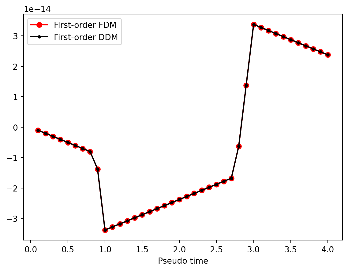
Next, we use the first-order sensitivity from the perturbed analysis to check the second-order derivative \(\frac{\partial^2 u}{\partial E^2}\):
FDMdudx2 = 1.0/(means[0]*perturbationFraction) * np.subtract(dudxPert[0], dudx[0])
plt.figure()
plt.plot(t, FDMdudx2, 'ro-', label='Second-order FDM')
plt.plot(t, dudx2[0, 0, :], 'ko-', label='Second-order DDM', markersize=3)
plt.xlabel("Pseudo time")
plt.legend(loc='lower left')
plt.show()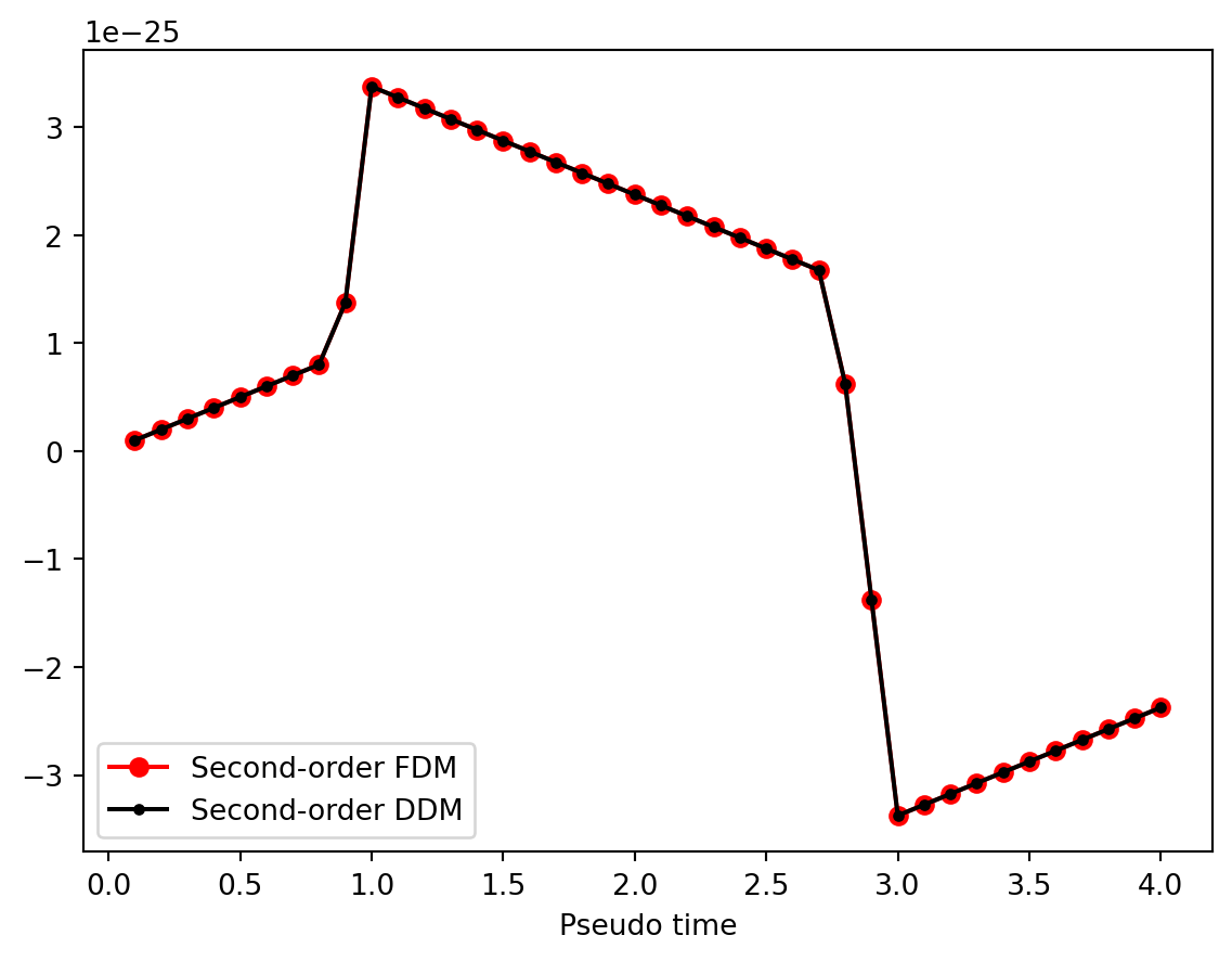
Again, a good match is observed. Proper implementation work requires greater care, both to examine all first- and second-order sensitivities and to carefully examine the value of discrepancies between finite difference and DDM calculations. That is done in background work for this book. More comprehensive examples are also provided on the website linked at the top of each chapter in this book.
14.3 Distributed Plasticity
The nonlinear portal frame analyzed in Chapter 9 is here re-created and plotted:
nel = 5
means, stdvs, distributions, correlation, trackNode, trackDOF, DDMs = nonlinearFrameVariableSpecs(nel)
input = createNonlinearFrameInput(*means, nel)
structuralModel = model(input)
structuralModel.plotModel()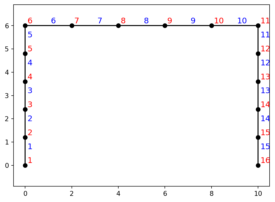
The analysis from that earlier chapter is re-run:
dt = 0.05
nsteps = 20
t, lamda, u, dudx, void = nonlinearStaticAnalysis(structuralModel, nsteps, dt, trackNode, trackDOF, DDMs, 1)
Following the pattern established above, the first input variable, i.e., the modulus of elasticity of the left-hand side column, is perturbed in order to get finite difference estimates of the first-order response sensitivity. A good match with the exact sensitivity is observed:
pertVar = means[0]*(1.0+perturbationFraction)
x = [pertVar, *means[1:]]
input = createNonlinearFrameInput(*x, nel)
structuralModel = model(input)
void, void, uPert, void, void = nonlinearStaticAnalysis(structuralModel, nsteps, dt, trackNode, trackDOF)
FDMdudx = 1.0/(means[0]*perturbationFraction) * np.subtract(uPert, u)
plt.figure()
plt.plot(t, FDMdudx, 'ro-', label='Finite difference')
plt.plot(t, dudx[0, :], 'ko-', label='DDM', markersize=3)
plt.xlabel("Pseudo time")
plt.legend(loc='lower left')
plt.show()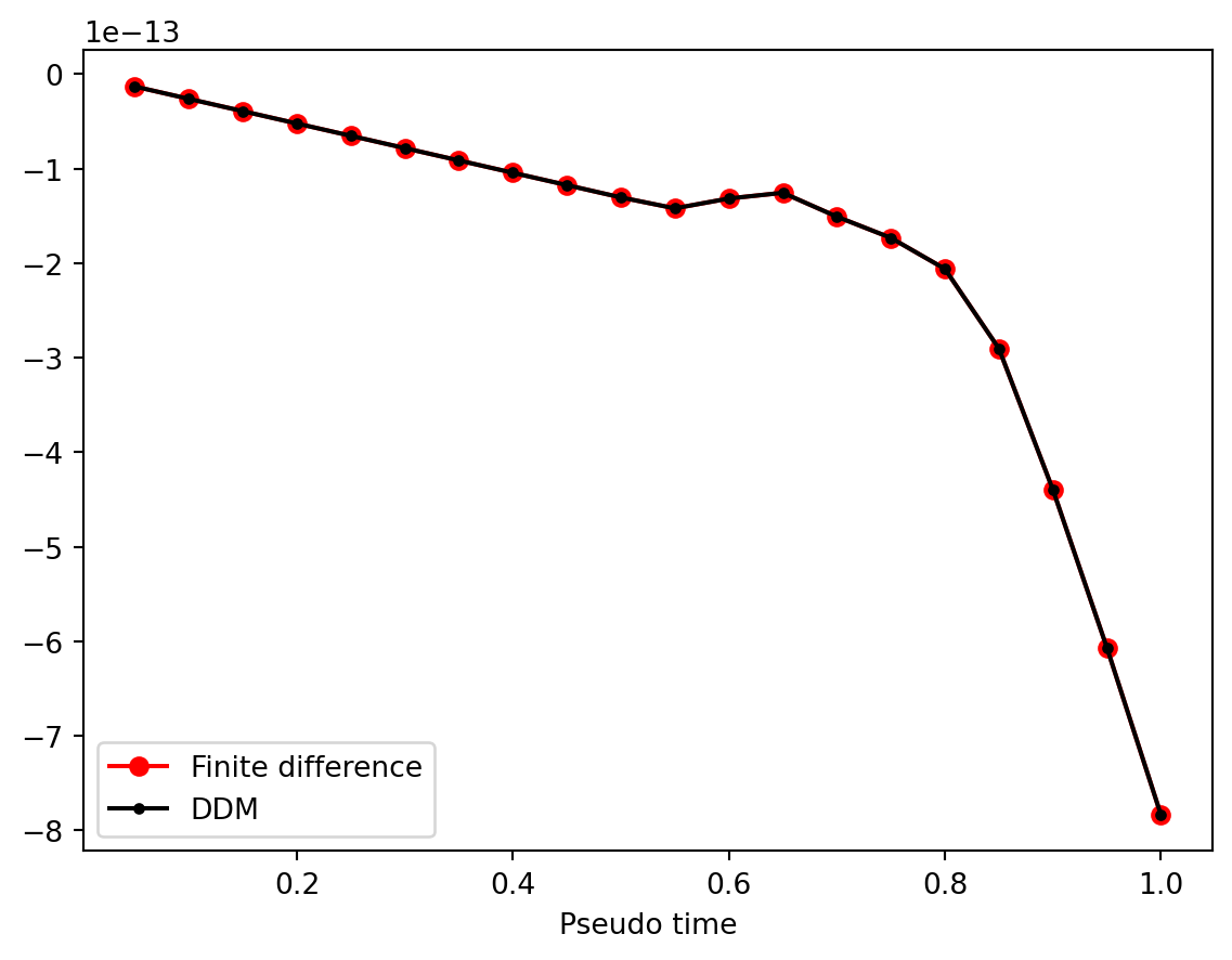
14.4 Linear Dynamics
The lumped mass column established in Section 10.4 and subjected to the El Centro ground motion in Section 10.14 is here re-created and plotted:
E = 200e9         # N/m^2
A = 18774e-6      # m^2 (W360X147 = W14x99)
I = 462016882e-12 # m^4
rho = 7850.0      # kg/m^3
nel = 5
input = createLinearColumnInput(E, A, I, rho, nel)
structuralModel = model(input)
structuralModel.plotModel()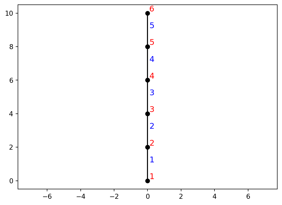
The analysis is also repeated, with sensitivity calculations:
trackNode = nel+1
trackDOF = 1
dampingModel = 'Rayleigh'
dampingRatio = 0.05
dM = [[0, 0, 0]]
for i in range(nel-1):
    dM.append([1, 0, 0])
dM.append([0.5, 0, 0])
DDMparameters = [['Element', 'E', range(1, nel+1)],
                 ['Node', 'M', dM],
                 ['Model', 'targetDamping']]
dt = 0.02
gmMatrix = readGroundMotion("ElCentro.txt", dt)
u, dudx = linearDynamicAnalysis(structuralModel, dampingModel, dampingRatio, gmMatrix, trackNode, trackDOF, DDMparameters)
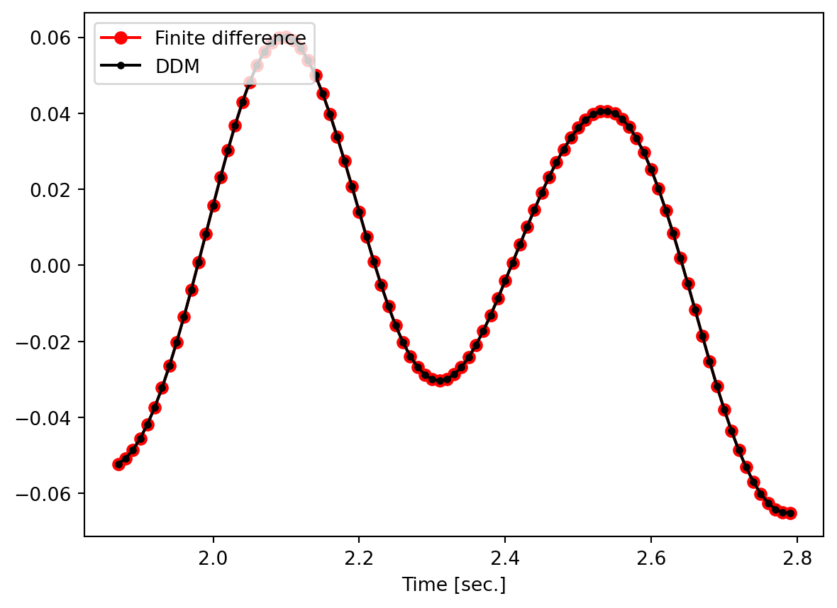
Next, the modulus of elasticity is perturbed and the corresponding response sensitivity is checked:
t = gmMatrix[0]
timeWindow = range(int(0.12*len(t)), int(0.18*len(t)))
pertE = E*(1.0+perturbationFraction)
x = [pertE, A, I, rho]
input = createLinearColumnInput(pertE, A, I, rho, nel)
structuralModel = model(input)
uPert, void = linearDynamicAnalysis(structuralModel, dampingModel, dampingRatio, gmMatrix, trackNode, trackDOF)
FDMdudx = 1.0/(E*perturbationFraction) * np.subtract(uPert, u)
plt.figure()
plt.plot(t[timeWindow], FDMdudx[timeWindow], 'ro-', label='Finite difference')
plt.plot(t[timeWindow], dudx[0, timeWindow], 'ko-', label='DDM', markersize=3)
plt.xlabel("Time [sec.]")
plt.legend(loc='upper right')
plt.show()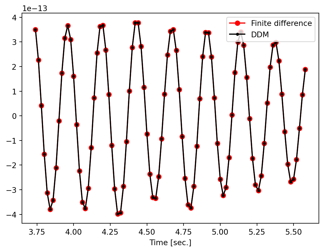
The same is here done for the damping ratio:
pertDampingRatio = dampingRatio*(1.0+perturbationFraction)
x = [E, A, I, rho]
input = createLinearColumnInput(E, A, I, rho, nel)
structuralModel = model(input)
uPert, void = linearDynamicAnalysis(structuralModel, dampingModel, pertDampingRatio, gmMatrix, trackNode, trackDOF)
FDMdudx = 1.0/(dampingRatio*perturbationFraction) * np.subtract(uPert, u)
plt.figure()
plt.plot(t[timeWindow], FDMdudx[timeWindow], 'ro-', label='Finite difference')
plt.plot(t[timeWindow], dudx[2, timeWindow], 'ko-', label='DDM', markersize=3)
plt.xlabel("Time [sec.]")
plt.legend(loc='upper right')
plt.show()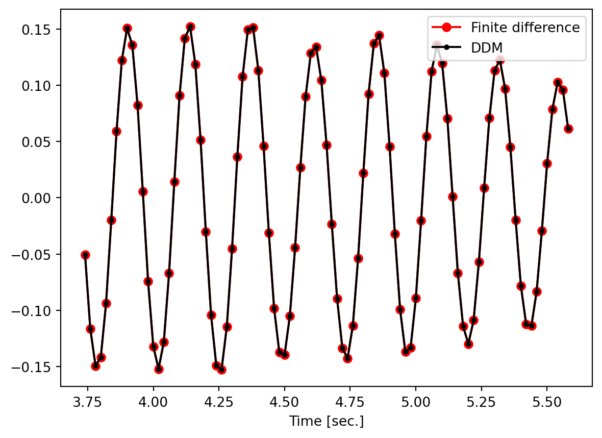
Next, the sensitivity of the response to change in the mass is checked:
L = 10
M = A * L/nel * rho
q = 0
NODES = []
for i in range(nel+1):
    NODES.append([0.0, i*L/nel])
CONSTRAINTS = [[1, 1, 1]]
for i in range(nel):
    CONSTRAINTS.append([0, 0, 0])
ELEMENTS = []
for i in range(nel):
    ELEMENTS.append([5, E, A, I, q, i+1, i+2])
SECTIONS = np.zeros(nel)
MATERIALS = np.zeros(nel)
LOADS = np.zeros((nel+1, 3))
pertMASS = [[0, 0, 0]]
for i in range(nel-1):
    pertMASS.append([M*(1.0+perturbationFraction), 0, 0])
pertMASS.append([0.5*M*(1.0+perturbationFraction), 0, 0])
input = [NODES, CONSTRAINTS, ELEMENTS, SECTIONS, MATERIALS, LOADS, pertMASS]
structuralModel = model(input)
uPert, void = linearDynamicAnalysis(structuralModel, dampingModel, dampingRatio, gmMatrix, trackNode, trackDOF)
FDMdudx = 1.0/(M*perturbationFraction) * np.subtract(uPert, u)
plt.figure()
plt.plot(t[timeWindow], FDMdudx[timeWindow], 'ro-', label='Finite difference')
plt.plot(t[timeWindow], dudx[1, timeWindow], 'ko-', label='DDM', markersize=3)
plt.xlabel("Time [sec.]")
plt.legend(loc='upper right')
plt.show()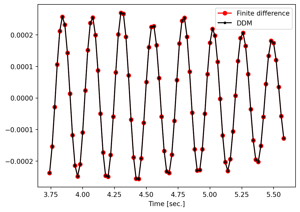
14.5 Nonlinear SDOF Dynamics
The analysis from Chapter 11 is here repeated:
Tn = 0.5      # seconds
E = 1e4       # N/m
alpha = 0.05  # Dimensionless
uy = 0.03     # m
fy = E * uy   # N
material = bilinearMaterial(['Bilinear', E, fy, alpha])
M = (Tn/2/np.pi)**2 * E
dampingRatio = 0.05
dt = 0.02
gmMatrix = readGroundMotion("ElCentro.txt", dt)
DDMparameters = [['Material', 'E'],
                 ['Material', 'fy'],
                 ['Material', 'alpha'],
                 ['Mass'],
                 ['Damping'],
                 ['GroundMotion', 'Scaling']]
t, u, v, a, dudx, dvdx, dadx, dudx2, dnl = nonlinearDynamicSDOFAnalysis(material, M, dampingRatio, gmMatrix, DDMparameters, 2)
Finite difference is here used to check \(\frac{\partial u}{\partial E}\):
pertE = E*(1.0+perturbationFraction)
material = bilinearMaterial(['Bilinear', pertE, fy, alpha])
void, uPert, void, void, void, void, void, void, void = nonlinearDynamicSDOFAnalysis(material, M, dampingRatio, gmMatrix)
FDMdudx = 1.0/(E*perturbationFraction) * np.subtract(uPert, u)
plt.figure()
plt.plot(t[timeWindow], FDMdudx[timeWindow], 'ro-', label='Finite difference')
plt.plot(t[timeWindow], dudx[0, timeWindow], 'ko-', label='DDM', markersize=3)
plt.xlabel("Time [sec.]")
plt.legend(loc='lower right')
plt.show()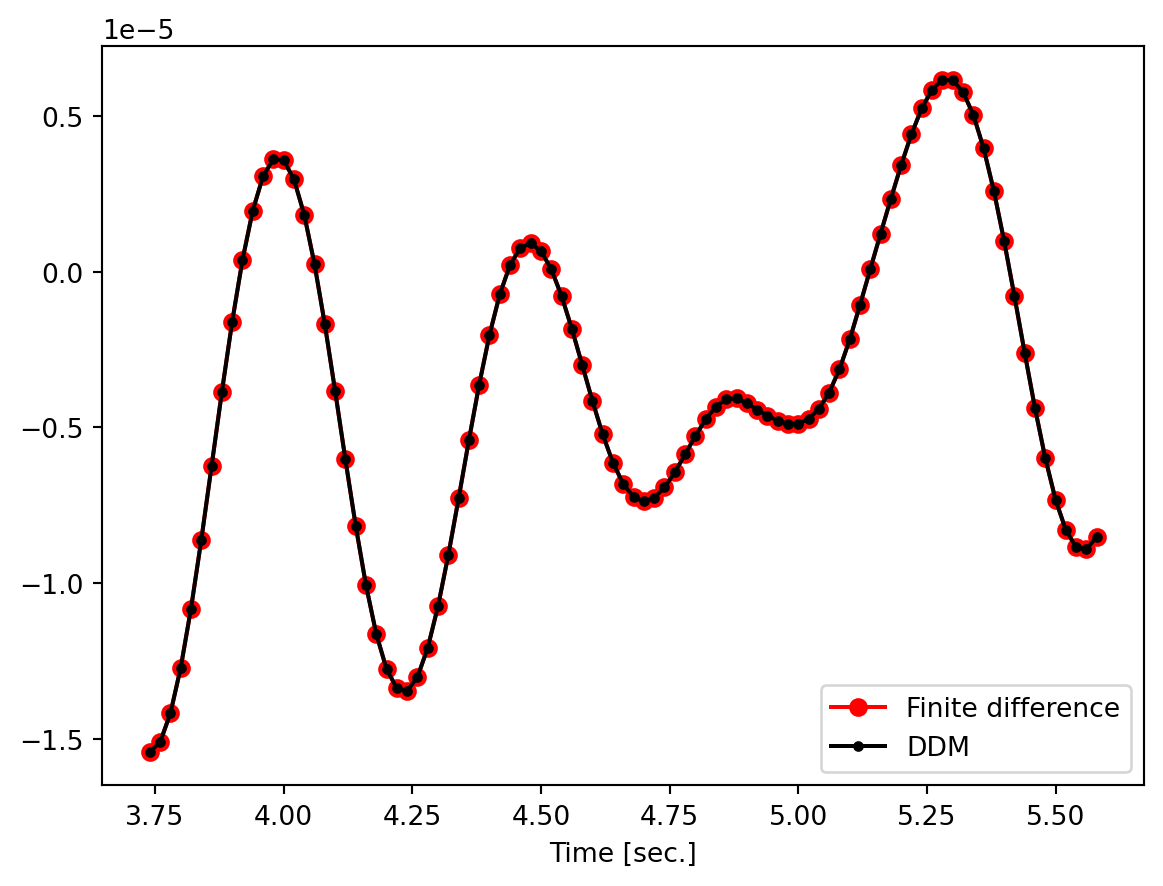
Finite difference is here used to check \(\frac{\partial u}{\partial f_y}\):
pertfy = fy*(1.0+perturbationFraction)
material = bilinearMaterial(['Bilinear', E, pertfy, alpha])
void, uPert, void, void, void, void, void, void, void = nonlinearDynamicSDOFAnalysis(material, M, dampingRatio, gmMatrix)
FDMdudx = 1.0/(fy*perturbationFraction) * np.subtract(uPert, u)
plt.figure()
plt.plot(t[timeWindow], FDMdudx[timeWindow], 'ro-', label='Finite difference')
plt.plot(t[timeWindow], dudx[1, timeWindow], 'ko-', label='DDM', markersize=3)
plt.xlabel("Time [sec.]")
plt.legend(loc='lower left')
plt.show()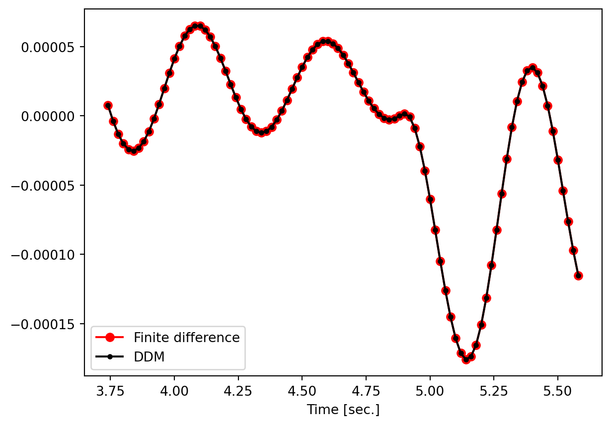
Finite difference is here used to check \(\frac{\partial u}{\partial \alpha}\):
pertAlpha = alpha*(1.0+perturbationFraction)
material = bilinearMaterial(['Bilinear', E, fy, pertAlpha])
void, uPert, void, void, void, void, void, void, void = nonlinearDynamicSDOFAnalysis(material, M, dampingRatio, gmMatrix)
FDMdudx = 1.0/(alpha*perturbationFraction) * np.subtract(uPert, u)
plt.figure()
plt.plot(t[timeWindow], FDMdudx[timeWindow], 'ro-', label='Finite difference')
plt.plot(t[timeWindow], dudx[2, timeWindow], 'ko-', label='DDM', markersize=3)
plt.xlabel("Time [sec.]")
plt.legend(loc='upper left')
plt.show()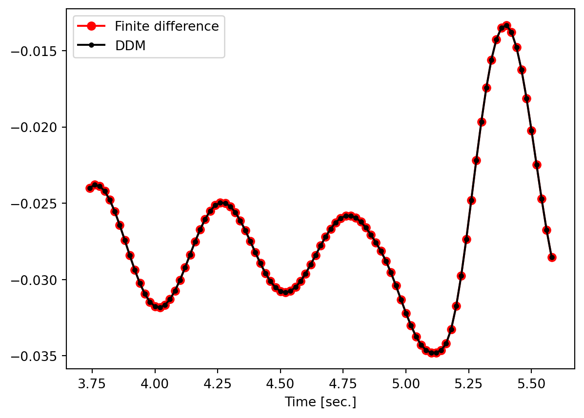
Finite difference is here used to check \(\frac{\partial u}{\partial M}\):
pertM = M*(1.0+perturbationFraction)
material = bilinearMaterial(['Bilinear', E, fy, alpha])
void, uPert, void, void, void, void, void, void, void = nonlinearDynamicSDOFAnalysis(material, pertM, dampingRatio, gmMatrix)
FDMdudx = 1.0/(M*perturbationFraction) * np.subtract(uPert, u)
plt.figure()
plt.plot(t[timeWindow], FDMdudx[timeWindow], 'ro-', label='Finite difference')
plt.plot(t[timeWindow], dudx[3, timeWindow], 'ko-', label='DDM', markersize=3)
plt.xlabel("Time [sec.]")
plt.legend(loc='upper right')
plt.show()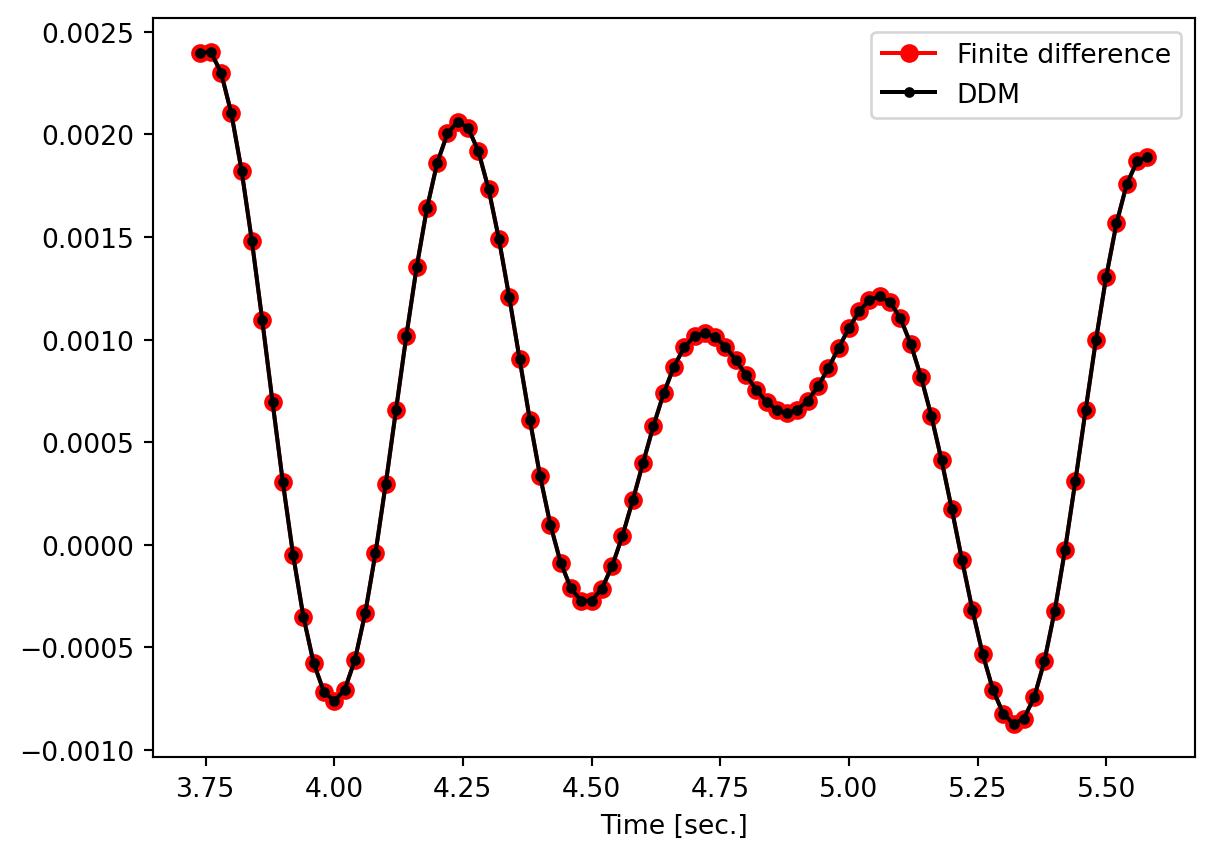
Finite difference is here used to check \(\frac{\partial u}{\partial \zeta}\):
pertDamping = dampingRatio*(1.0+perturbationFraction)
material = bilinearMaterial(['Bilinear', E, fy, alpha])
void, uPert, void, void, void, void, void, void, void = nonlinearDynamicSDOFAnalysis(material, M, pertDamping, gmMatrix)
FDMdudx = 1.0/(dampingRatio*perturbationFraction) * np.subtract(uPert, u)
plt.figure()
plt.plot(t[timeWindow], FDMdudx[timeWindow], 'ro-', label='Finite difference')
plt.plot(t[timeWindow], dudx[4, timeWindow], 'ko-', label='DDM', markersize=3)
plt.xlabel("Time [sec.]")
plt.legend(loc='lower right')
plt.show()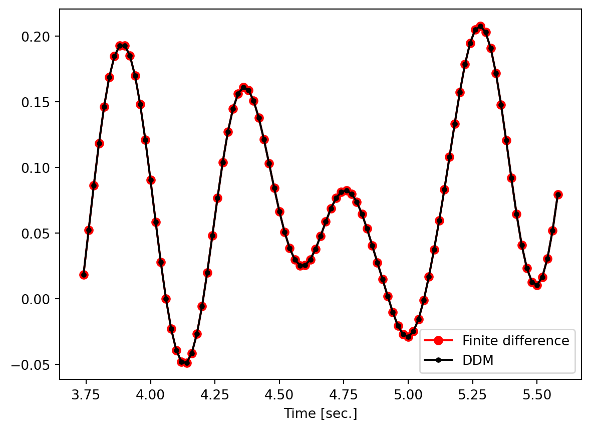
Finite difference is here used to check \(\frac{\partial u}{\partial s}\):
material = bilinearMaterial(['Bilinear', E, fy, alpha])
pertGM = np.concatenate(([gmMatrix[0]], [np.multiply(gmMatrix[1], 1.0+perturbationFraction)]), axis=0)
void, uPert, void, void, void, void, void, void, void = nonlinearDynamicSDOFAnalysis(material, M, dampingRatio, pertGM)
FDMdudx = 1.0/(perturbationFraction) * np.subtract(uPert, u)
plt.figure()
plt.plot(t[timeWindow], FDMdudx[timeWindow], 'ro-', label='Finite difference')
plt.plot(t[timeWindow], dudx[5, timeWindow], 'ko-', label='DDM', markersize=3)
plt.xlabel("Time [sec.]")
plt.legend(loc='lower right')
plt.show()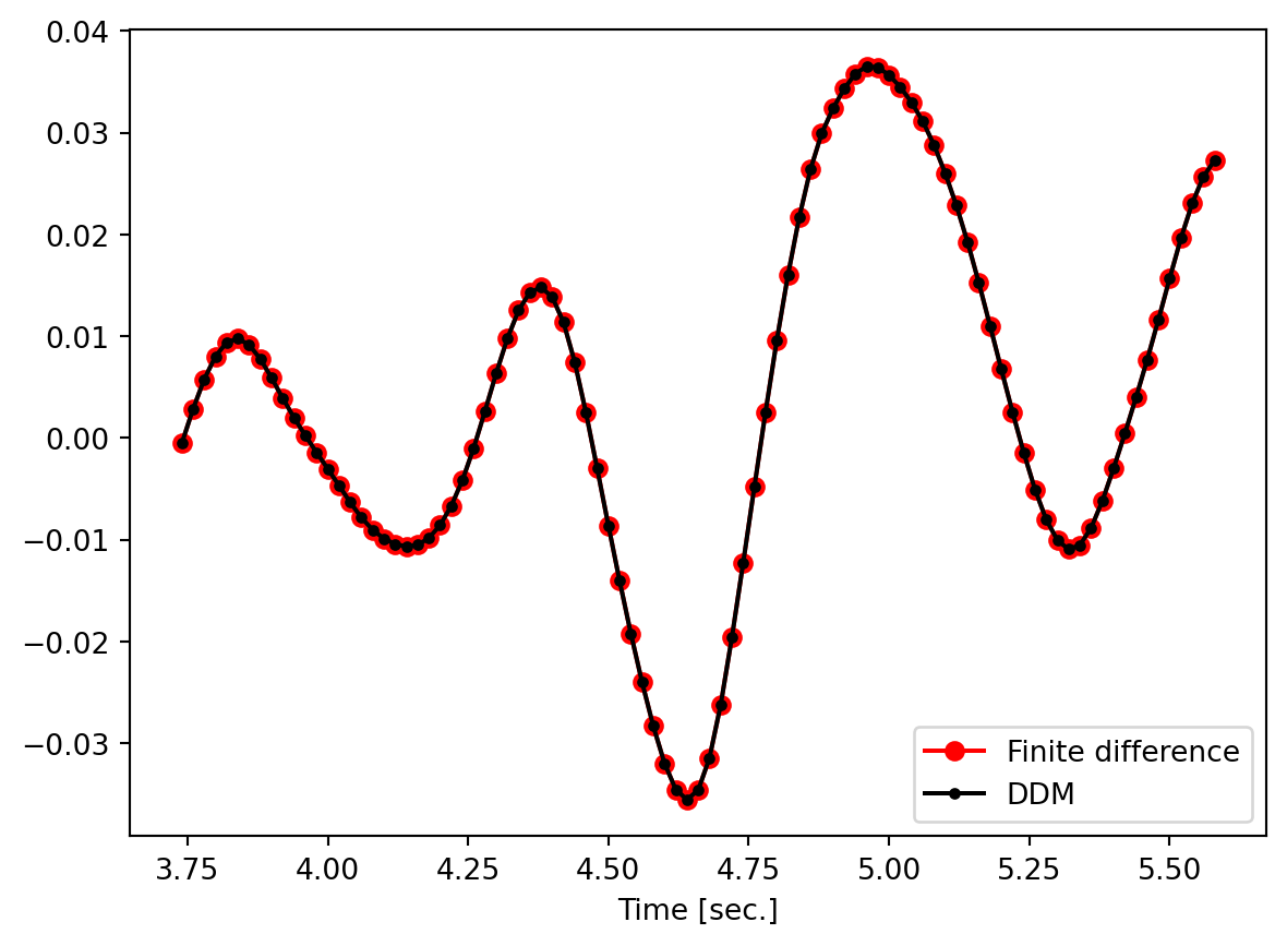
14.6 Nonlinear MDOF Dynamics
The nonlinear column model from Chapter 12 is here re-created and plotted:
nel = 5
means, stdvs, distributions, correlation, trackNode, trackDOF, DDMs = nonlinearColumnVariableSpecs(nel)
input = createNonlinearColumnInput(*means, nel)
structuralModel = model(input)
structuralModel.plotModel()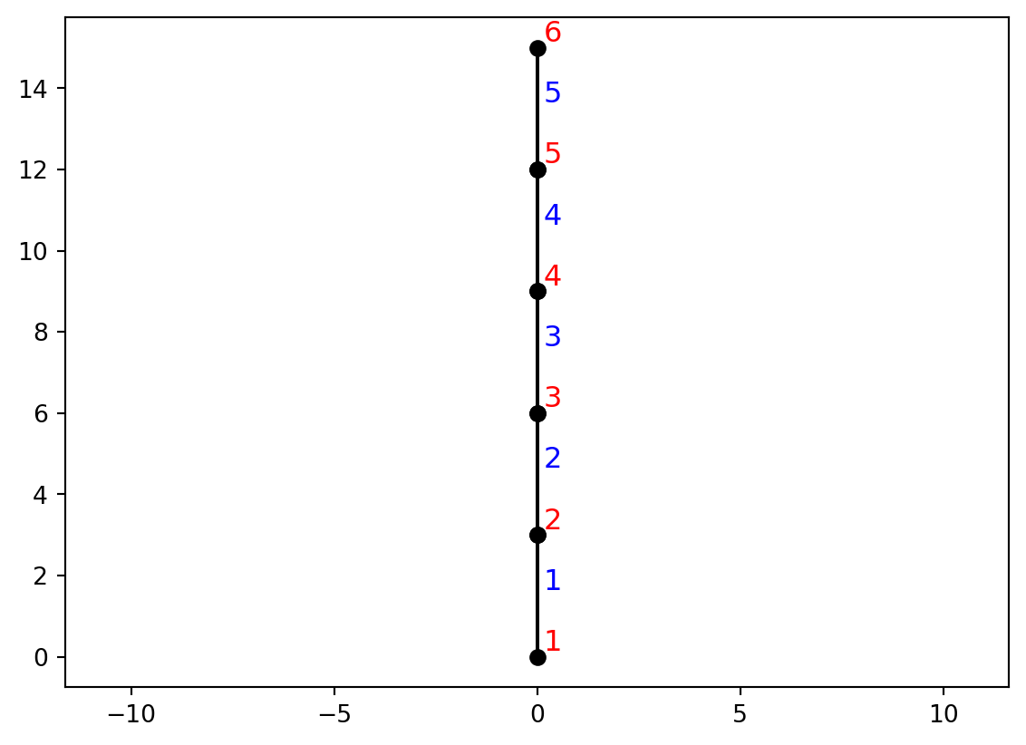
Next, the analysis is re-run, here with Rayleigh damping using the tangent stiffness matrix and proportionality coefficients continuously updated during the analysis, also based on the tangent stiffness:
targetDamping = 0.05
dampingMT = ['Modal', 'Current', targetDamping]
dampingRTi = ['Rayleigh', 'Current', 'Initial', 1, 2, targetDamping]
dampingRTt = ['Rayleigh', 'Current', 'Current', 1, 2, targetDamping]
dampingModel = dampingRTt
dt = 0.005
t = np.arange(0, 2, dt)
groundAcceleration = np.zeros(len(t))
for i in range(len(t)):
    if t[i] <= 0.5:
        groundAcceleration[i] = 5 * 9.81 * np.sin(2 * np.pi * t[i])
gmMatrix = np.concatenate(([t], [groundAcceleration]), axis=0)
t, gm, u, v, a, dudx, dvdx, dadx, dnl1, dnl2 = nonlinearDynamicAnalysis(structuralModel, dampingModel, gmMatrix, trackNode, trackDOF, 1, DDMs)
Finite difference is here used to check \(\frac{\partial u}{\partial E}\):
pertE = means[0]*(1.0+perturbationFraction)
x = [pertE, *means[1:]]
input = createNonlinearColumnInput(*x, nel)
structuralModel = model(input)
void, void, uPert, void, void, void, void, void, void, void = nonlinearDynamicAnalysis(structuralModel, dampingModel, gmMatrix, trackNode, trackDOF)
FDMdudx = 1.0/(means[0]*perturbationFraction) * np.subtract(uPert[0,:], u[0,:])
plt.figure()
plt.plot(t, FDMdudx, 'ro-', label='Finite difference')
plt.plot(t, dudx[0, 0, :], 'ko-', label='DDM', markersize=3)
plt.xlabel("Time [sec.]")
plt.legend(loc='upper left')
plt.grid(True)
plt.show()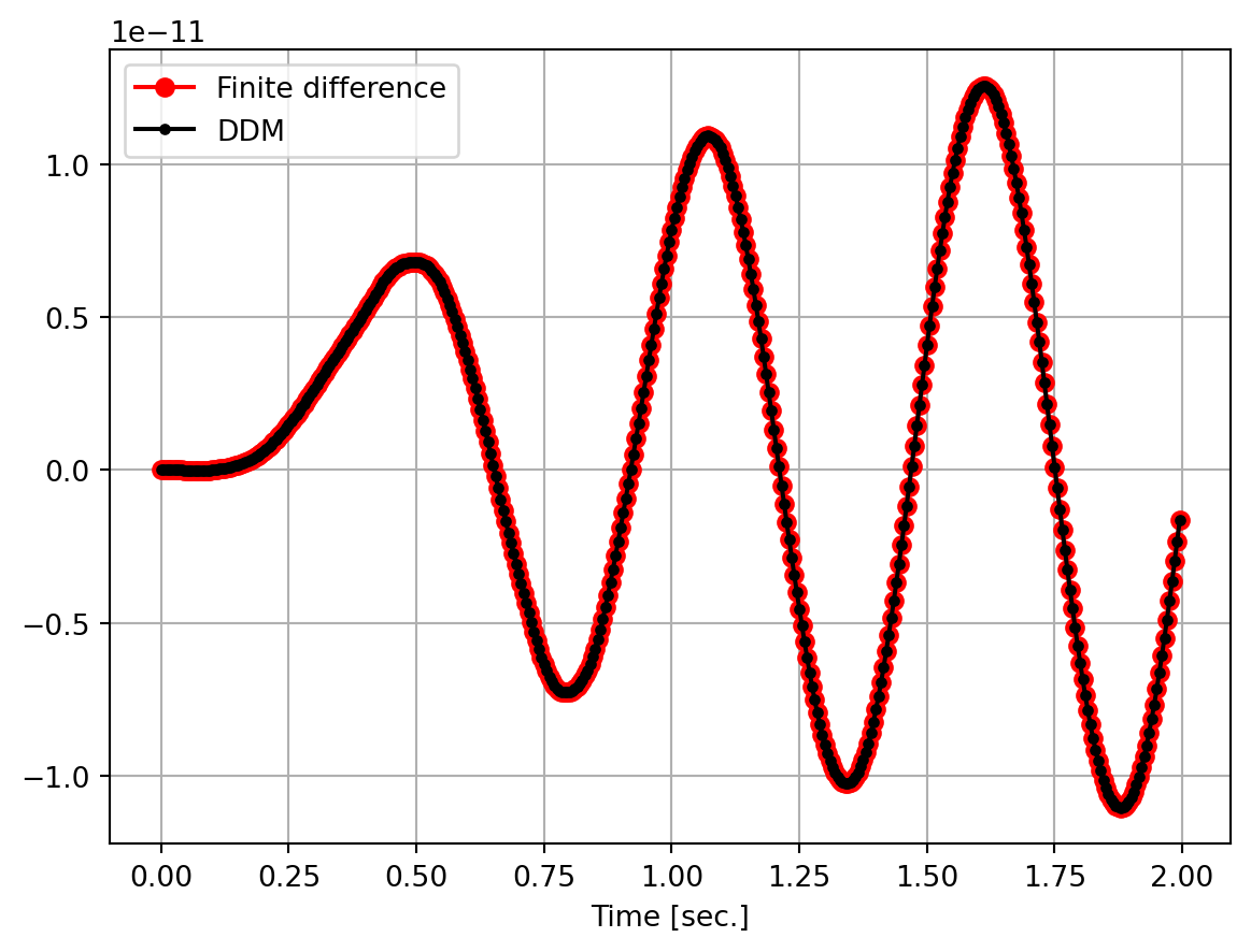
The code above is easily modified to check the sensitivity to other variables. That is done in code posted on the website linked at the top of each chapter of this book.
14.7 Synthetic Ground Motions
The next three subsections verify the following sensitivity calculations:
- \(\frac{\partial \ddot{u}_g}{\partial \sigma_g}\), \(\frac{\partial \ddot{u}_g}{\partial \omega_g}\), and \(\frac{\partial \ddot{u}_g}{\partial \zeta_g}\) for the spectral approach to generating ground motions
- \(\frac{\partial \ddot{u}_g}{\partial \sigma_g}\), \(\frac{\partial \ddot{u}_g}{\partial \omega_g}\), and \(\frac{\partial \ddot{u}_g}{\partial \zeta_g}\) for the filtered white noise approach to generating ground motions
- \(\frac{\partial u}{\partial \sigma_g}\), \(\frac{\partial u}{\partial \omega_g}\), and \(\frac{\partial u}{\partial \zeta_g}\), i.e., structural response sensitivities, for the spectral approach to generating ground motions
- \(\frac{\partial u}{\partial \sigma_g}\), \(\frac{\partial u}{\partial \omega_g}\), and \(\frac{\partial u}{\partial \zeta_g}\), i.e., structural response sensitivities, for the filtered white noise approach to generating ground motions
14.7.1 Spectral
These are the parameters specified for all the ground motions generated in this section:
sigma_g = 2/1.75
omega_g = 15
zeta_g = omega_g/25
minFreq = 0
maxFreq = 5*omega_g
nblocks = 200
omega = np.linspace(minFreq, maxFreq, nblocks)
seed = 1
duration = 25.0
dt = 0.01
t1 = 0
t2 = 3
t3 = 10
t4 = duration
Based on those parameters, the spectral ground motion is generated here:
gmMatrix = spectralGroundMotion(duration, dt, minFreq, maxFreq, nblocks, sigma_g, omega_g, zeta_g, trapezoidalModulatingFunction, t1, t2, t3, t4, seed)Here is the check of \(\frac{\partial \ddot{u}_g}{\partial \sigma_g}\):
pertMatrix = spectralGroundMotion(duration, dt, minFreq, maxFreq, nblocks, sigma_g*(1+perturbationFraction), omega_g, zeta_g, trapezoidalModulatingFunction, t1, t2, t3, t4, seed)
dGMdSigma = (pertMatrix[1]-gmMatrix[1])/(sigma_g*perturbationFraction)
plt.figure()
plt.plot(gmMatrix[0, timeWindow], dGMdSigma[timeWindow], 'ro-', label='Finite difference')
plt.plot(gmMatrix[0, timeWindow], gmMatrix[2, timeWindow], 'ko-', label='DDM', markersize=3)
plt.xlabel("Time [sec.]")
plt.legend(loc='upper right')
plt.show()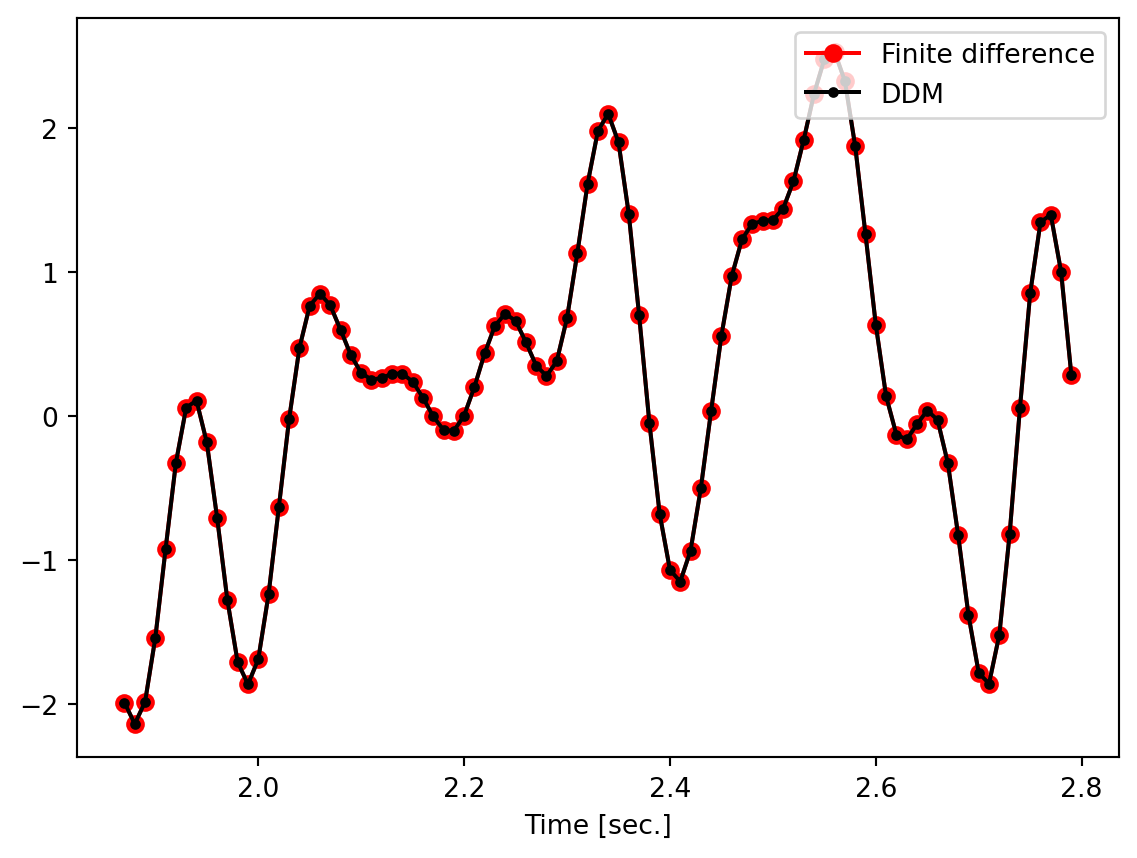
Here is the check of \(\frac{\partial \ddot{u}_g}{\partial \omega_g}\):
pertMatrix = spectralGroundMotion(duration, dt, minFreq, maxFreq, nblocks, sigma_g, omega_g*(1+perturbationFraction), zeta_g, trapezoidalModulatingFunction, t1, t2, t3, t4, seed)
dGMdOmega = (pertMatrix[1]-gmMatrix[1])/(omega_g*perturbationFraction)
plt.figure()
plt.plot(gmMatrix[0, timeWindow], dGMdOmega[timeWindow], 'ro-', label='Finite difference')
plt.plot(gmMatrix[0, timeWindow], gmMatrix[3, timeWindow], 'ko-', label='DDM', markersize=3)
plt.xlabel("Time [sec.]")
plt.legend(loc='upper right')
plt.show()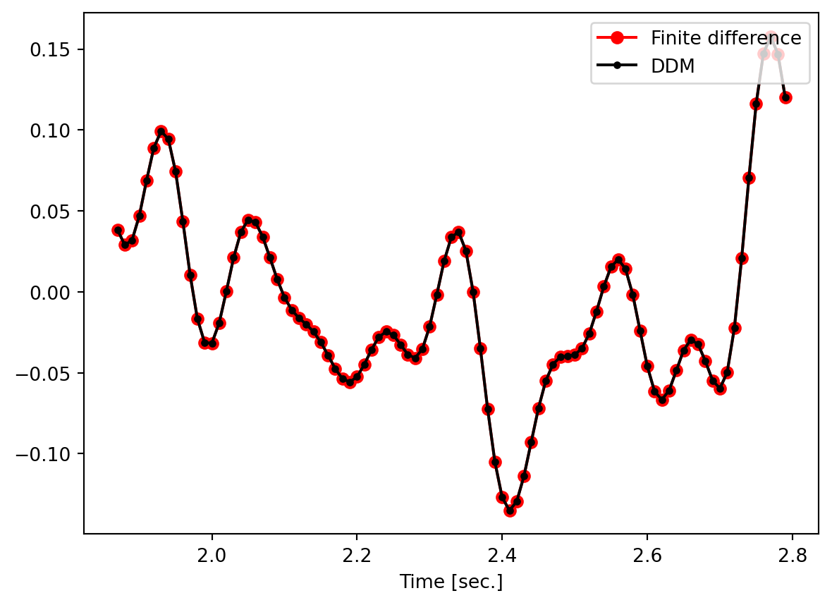
Here is the check of \(\frac{\partial \ddot{u}_g}{\partial \zeta_g}\):
pertMatrix = spectralGroundMotion(duration, dt, minFreq, maxFreq, nblocks, sigma_g, omega_g, zeta_g*(1+perturbationFraction), trapezoidalModulatingFunction, t1, t2, t3, t4, seed)
dGMdZeta = (pertMatrix[1]-gmMatrix[1])/(zeta_g*perturbationFraction)
plt.figure()
plt.plot(gmMatrix[0, timeWindow], dGMdZeta[timeWindow], 'ro-', label='Finite difference')
plt.plot(gmMatrix[0, timeWindow], gmMatrix[4, timeWindow], 'ko-', label='DDM', markersize=3)
plt.xlabel("Time [sec.]")
plt.legend(loc='upper right')
plt.show()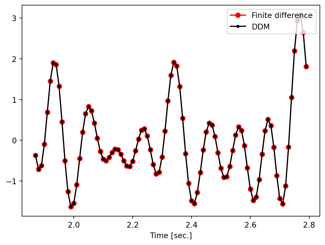
14.7.2 Filtered White Noise
Based on the parameters specified above, the filtered white noise ground motion is generated here:
scaling = 4
pulseRate = 10
gmMatrix = filteredWhiteNoise(duration, dt, scaling, sigma_g, omega_g, zeta_g, pulseRate, trapezoidalModulatingFunction, t1, t2, t3, t4, seed)
Here is the check of \(\frac{\partial \ddot{u}_g}{\partial \sigma_g}\):
pertMatrix = filteredWhiteNoise(duration, dt, scaling, sigma_g*(1+perturbationFraction), omega_g, zeta_g, pulseRate, trapezoidalModulatingFunction, t1, t2, t3, t4, seed)
dGMdSigma = (pertMatrix[1]-gmMatrix[1])/(sigma_g*perturbationFraction)
plt.figure()
plt.plot(gmMatrix[0, timeWindow], dGMdSigma[timeWindow], 'ro-', label='Finite difference')
plt.plot(gmMatrix[0, timeWindow], gmMatrix[2, timeWindow], 'ko-', label='DDM', markersize=3)
plt.xlabel("Time [sec.]")
plt.legend(loc='upper left')
plt.show()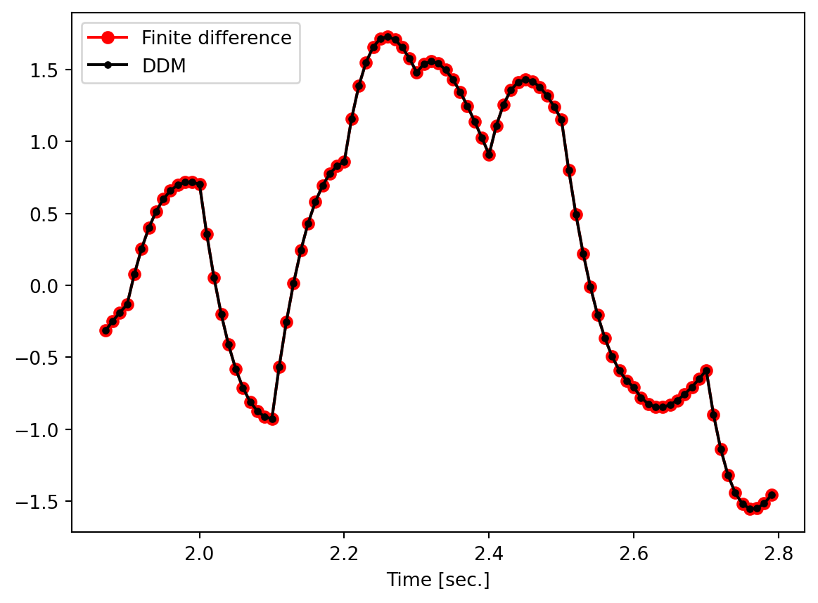
Here is the check of \(\frac{\partial \ddot{u}_g}{\partial \omega_g}\):
pertMatrix = filteredWhiteNoise(duration, dt, scaling, sigma_g, omega_g*(1+perturbationFraction), zeta_g, pulseRate, trapezoidalModulatingFunction, t1, t2, t3, t4, seed)
dGMdOmega = (pertMatrix[1]-gmMatrix[1])/(omega_g*perturbationFraction)
plt.figure()
plt.plot(gmMatrix[0, timeWindow], dGMdOmega[timeWindow], 'ro-', label='Finite difference')
plt.plot(gmMatrix[0, timeWindow], gmMatrix[3, timeWindow], 'ko-', label='DDM', markersize=3)
plt.xlabel("Time [sec.]")
plt.legend(loc='upper left')
plt.show()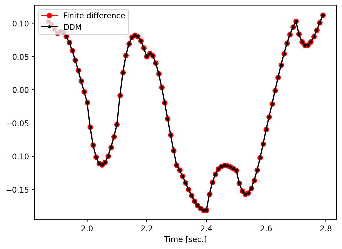
Here is the check of \(\frac{\partial \ddot{u}_g}{\partial \zeta_g}\):
pertMatrix = filteredWhiteNoise(duration, dt, scaling, sigma_g, omega_g, zeta_g*(1+perturbationFraction), pulseRate, trapezoidalModulatingFunction, t1, t2, t3, t4, seed)
dGMdZeta = (pertMatrix[1]-gmMatrix[1])/(zeta_g*perturbationFraction)
plt.figure()
plt.plot(gmMatrix[0, timeWindow], dGMdZeta[timeWindow], 'ro-', label='Finite difference')
plt.plot(gmMatrix[0, timeWindow], gmMatrix[4, timeWindow], 'ko-', label='DDM', markersize=3)
plt.xlabel("Time [sec.]")
plt.legend(loc='upper left')
plt.show()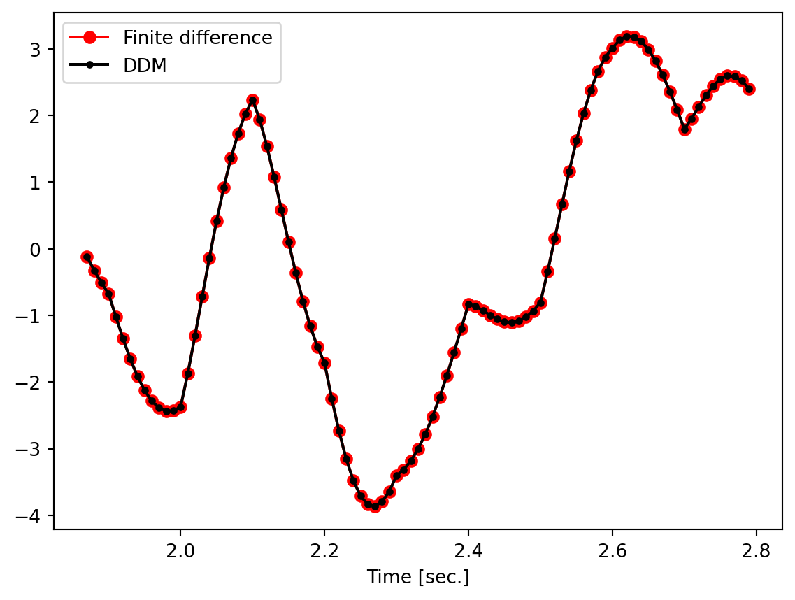
14.7.3 Structural Response
The “structure” considered here is a single-DOF system with these specifications:
Tn = 0.5      # seconds
E = 1e4       # N/m
alpha = 0.05  # Dimensionless
uy = 0.03     # m
fy = E * uy   # N
material = bilinearMaterial(['Bilinear', E, fy, alpha])
M = (Tn/2/np.pi)**2 * E
dampingRatio = 0.05
DDMparameters = [['GroundMotion', 'GivenDerivative', 1],
                 ['GroundMotion', 'GivenDerivative', 2],
                 ['GroundMotion', 'GivenDerivative', 3]]
The spectral ground motion is here generated and the nonlinear dynamic analysis is re-run:
gmMatrix = spectralGroundMotion(duration, dt, minFreq, maxFreq, nblocks, sigma_g, omega_g, zeta_g, trapezoidalModulatingFunction, t1, t2, t3, t4, seed)
material = bilinearMaterial(['Bilinear', E, fy, alpha])
t, u, v, a, dudx, dvdx, dadx, dudx2, dnl = nonlinearDynamicSDOFAnalysis(material, M, dampingRatio, gmMatrix, DDMparameters, 1)
Here is the check of \(\frac{\partial u}{\partial \sigma_g}\):
material = bilinearMaterial(['Bilinear', E, fy, alpha])
pertMatrix1 = spectralGroundMotion(duration, dt, minFreq, maxFreq, nblocks, sigma_g*(1+perturbationFraction), omega_g, zeta_g, trapezoidalModulatingFunction, t1, t2, t3, t4, seed)
void, uPert, void, void, void, void, void, void, void = nonlinearDynamicSDOFAnalysis(material, M, dampingRatio, pertMatrix1)
FDMdudx = 1.0/(sigma_g*perturbationFraction) * np.subtract(uPert, u)
plt.figure()
plt.plot(t[timeWindow], FDMdudx[timeWindow], 'ro-', label='Finite difference')
plt.plot(t[timeWindow], dudx[0, timeWindow], 'ko-', label='DDM', markersize=3)
plt.xlabel("Time [sec.]")
plt.legend(loc='lower left')
plt.show()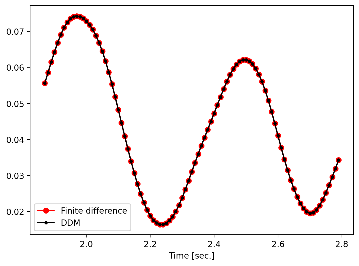
Here is the check of \(\frac{\partial u}{\partial \omega_g}\):
material = bilinearMaterial(['Bilinear', E, fy, alpha])
pertMatrix2 = spectralGroundMotion(duration, dt, minFreq, maxFreq, nblocks, sigma_g, omega_g*(1+perturbationFraction), zeta_g, trapezoidalModulatingFunction, t1, t2, t3, t4, seed)
void, uPert, void, void, void, void, void, void, void = nonlinearDynamicSDOFAnalysis(material, M, dampingRatio, pertMatrix2)
FDMdudx = 1.0/(omega_g*perturbationFraction) * np.subtract(uPert, u)
plt.figure()
plt.plot(t[timeWindow], FDMdudx[timeWindow], 'ro-', label='Finite difference')
plt.plot(t[timeWindow], dudx[1, timeWindow], 'ko-', label='DDM', markersize=3)
plt.xlabel("Time [sec.]")
plt.legend(loc='upper left')
plt.show()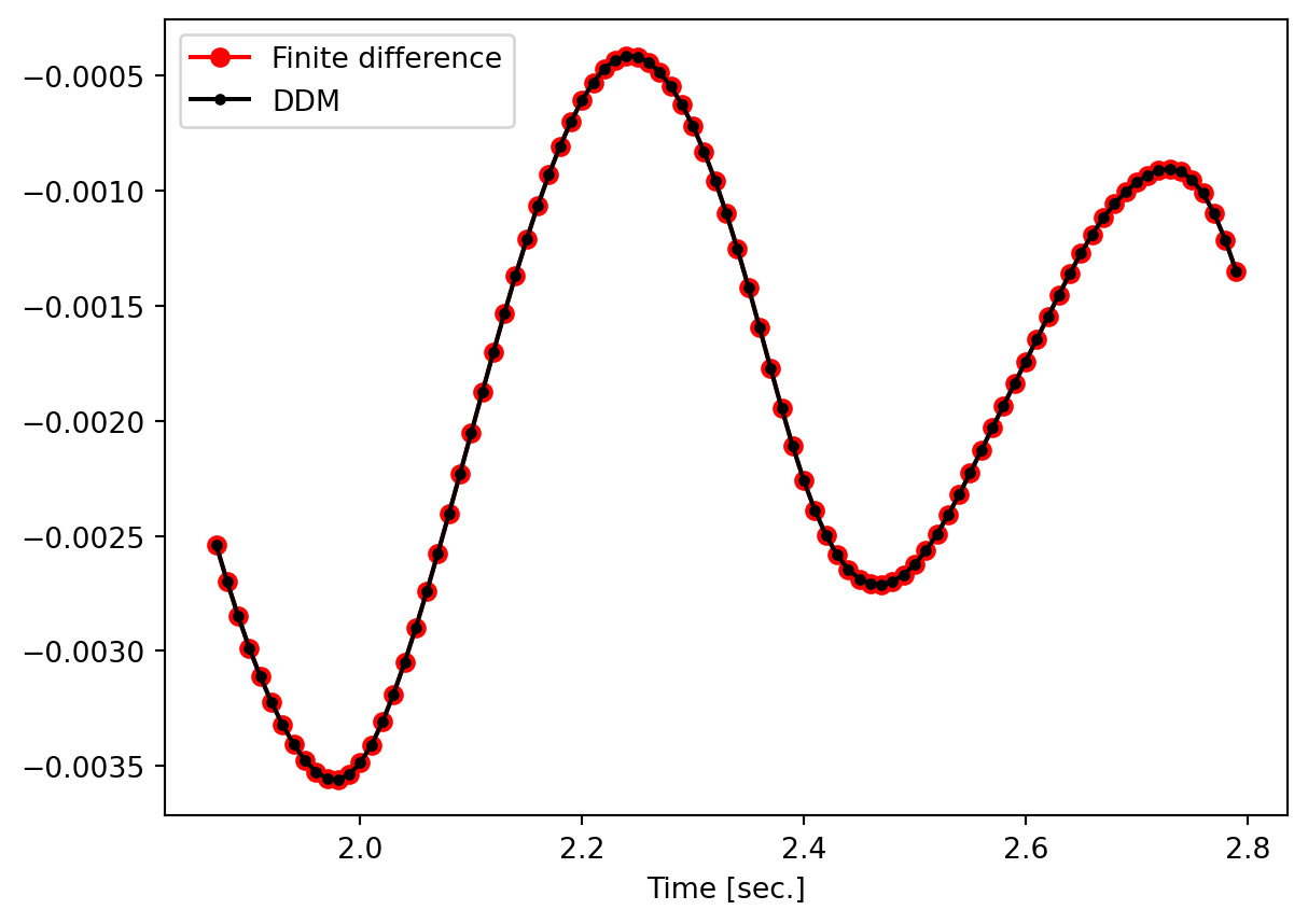
Here is the check of \(\frac{\partial u}{\partial \zeta_g}\):
material = bilinearMaterial(['Bilinear', E, fy, alpha])
pertMatrix3 = spectralGroundMotion(duration, dt, minFreq, maxFreq, nblocks, sigma_g, omega_g, zeta_g*(1+perturbationFraction), trapezoidalModulatingFunction, t1, t2, t3, t4, seed)
void, uPert, void, void, void, void, void, void, void = nonlinearDynamicSDOFAnalysis(material, M, dampingRatio, pertMatrix3)
FDMdudx = 1.0/(zeta_g*perturbationFraction) * np.subtract(uPert, u)
plt.figure()
plt.plot(t[timeWindow], FDMdudx[timeWindow], 'ro-', label='Finite difference')
plt.plot(t[timeWindow], dudx[2, timeWindow], 'ko-', label='DDM', markersize=3)
plt.xlabel("Time [sec.]")
plt.legend(loc='upper left')
plt.show()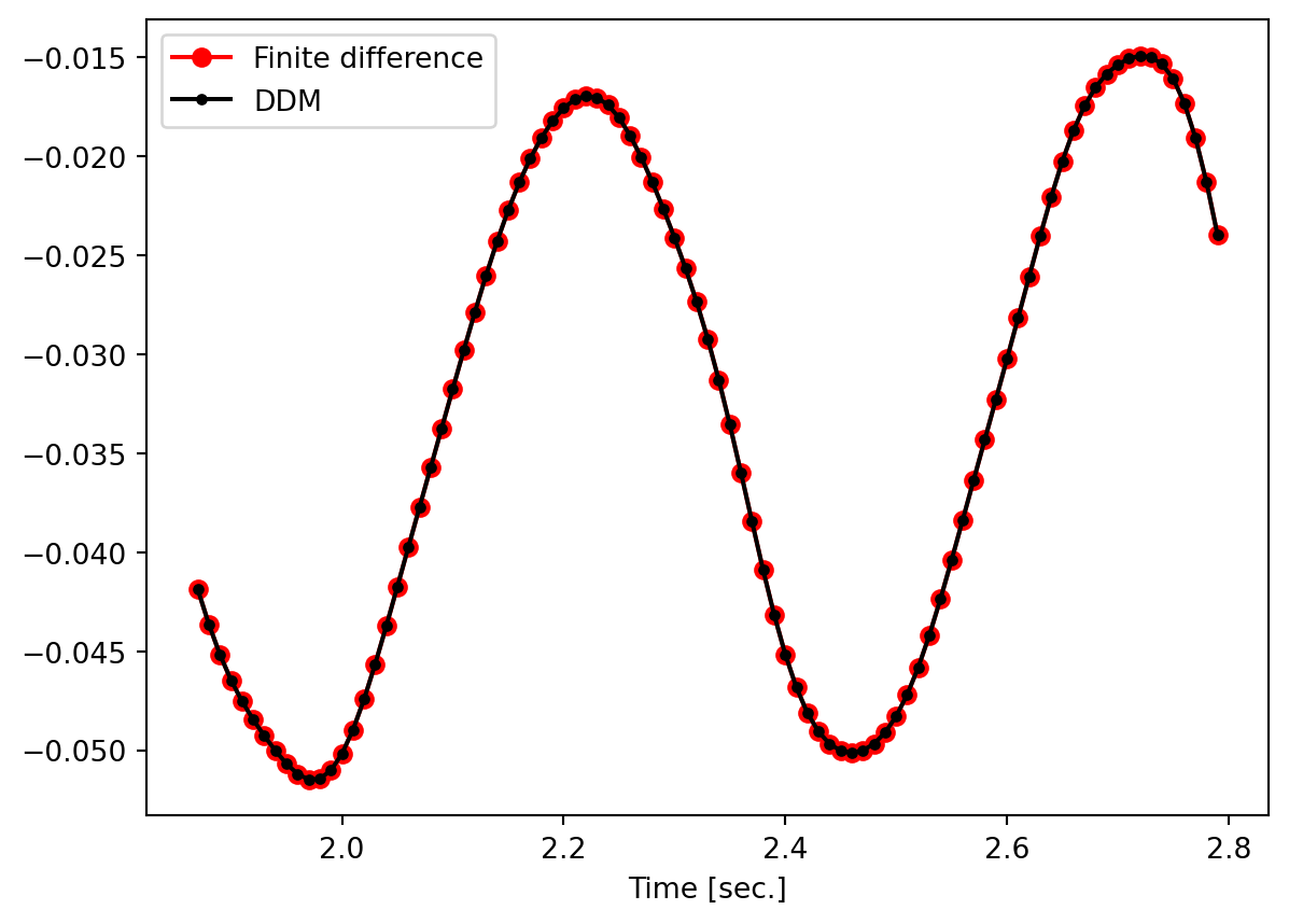
The filtered white noise ground motion is here generated and the nonlinear dynamic analysis is re-run:
gmMatrix = filteredWhiteNoise(duration, dt, scaling, sigma_g, omega_g, zeta_g, pulseRate, trapezoidalModulatingFunction, t1, t2, t3, t4, seed)
material = bilinearMaterial(['Bilinear', E, fy, alpha])
t, u, v, a, dudx, dvdx, dadx, dudx2, dnl = nonlinearDynamicSDOFAnalysis(material, M, dampingRatio, gmMatrix, DDMparameters, 1)
Here is the check of \(\frac{\partial u}{\partial \sigma_g}\):
material = bilinearMaterial(['Bilinear', E, fy, alpha])
pertMatrix1 = filteredWhiteNoise(duration, dt, scaling, sigma_g*(1+perturbationFraction), omega_g, zeta_g, pulseRate, trapezoidalModulatingFunction, t1, t2, t3, t4, seed)
void, uPert, void, void, void, void, void, void, void = nonlinearDynamicSDOFAnalysis(material, M, dampingRatio, pertMatrix1)
FDMdudx = 1.0/(sigma_g*perturbationFraction) * np.subtract(uPert, u)
plt.figure()
plt.plot(t[timeWindow], FDMdudx[timeWindow], 'ro-', label='Finite difference')
plt.plot(t[timeWindow], dudx[0, timeWindow], 'ko-', label='DDM', markersize=3)
plt.xlabel("Time [sec.]")
plt.legend(loc='lower left')
plt.show()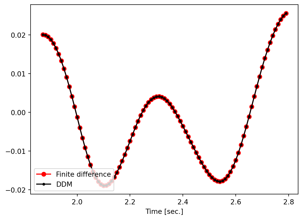
Here is the check of \(\frac{\partial u}{\partial \omega_g}\):
material = bilinearMaterial(['Bilinear', E, fy, alpha])
pertMatrix2 = filteredWhiteNoise(duration, dt, scaling, sigma_g, omega_g*(1+perturbationFraction), zeta_g, pulseRate, trapezoidalModulatingFunction, t1, t2, t3, t4, seed)
void, uPert, void, void, void, void, void, void, void = nonlinearDynamicSDOFAnalysis(material, M, dampingRatio, pertMatrix2)
FDMdudx = 1.0/(omega_g*perturbationFraction) * np.subtract(uPert, u)
plt.figure()
plt.plot(t[timeWindow], FDMdudx[timeWindow], 'ro-', label='Finite difference')
plt.plot(t[timeWindow], dudx[1, timeWindow], 'ko-', label='DDM', markersize=3)
plt.xlabel("Time [sec.]")
plt.legend(loc='upper left')
plt.show()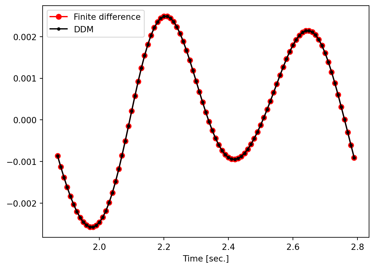
Here is the check of \(\frac{\partial u}{\partial \zeta_g}\):
material = bilinearMaterial(['Bilinear', E, fy, alpha])
pertMatrix3 = filteredWhiteNoise(duration, dt, scaling, sigma_g, omega_g, zeta_g*(1+perturbationFraction), pulseRate, trapezoidalModulatingFunction, t1, t2, t3, t4, seed)
void, uPert, void, void, void, void, void, void, void = nonlinearDynamicSDOFAnalysis(material, M, dampingRatio, pertMatrix3)
FDMdudx = 1.0/(zeta_g*perturbationFraction) * np.subtract(uPert, u)
plt.figure()
plt.plot(t[timeWindow], FDMdudx[timeWindow], 'ro-', label='Finite difference')
plt.plot(t[timeWindow], dudx[2, timeWindow], 'ko-', label='DDM', markersize=3)
plt.xlabel("Time [sec.]")
plt.legend(loc='upper left')
plt.show()