from Chapter4code import *5 Reliability Algorithms
The development of reliability methods, addressing the problem defined in Section 1.9, follows an interesting trajectory. In a nutshell, it starts with the invention of the reliability index by Cornell (1969) and culminates with the seminal textbook by Der Kiureghian (2022). Papers published in the mid-1970s and work in the 1980s also contribute significantly to the limit-state design embedded in present-day building codes and design standards.
5.1 Reliability Index
The reliability index, \(\beta\), represents an alternative to working with the failure probability, \(p_f\). Simply put, \(\beta\) is the number of standard deviations from the mean realization of the input variables to failure. Applicable to linear limit-state functions, Professor Cornell introduced its definition as
\[ \beta = \frac{\mu_g}{\sigma_g} \tag{5.1}\]
where \(\mu_g\) and \(\sigma_g\) are the mean and standard deviation of the limit-state function, which was defined in Section 1.10. Holding on to the thought that \(g\) is a random variable in its own right, the definition in Equation 5.1, which implies \(\mu_g = \beta\cdot \sigma_g\), does indeed say that the mean is \(\beta\) standard deviations away from \(g=0\), which is the border between fail and safe.
\(\mu_g\) and \(\sigma_g\) are calculated with the first-order approximations given in Chapter 4. That means they are exact if the limit-state function, \(g(\mathbf{x})\), is a linear function of \(\mathbf{x}\). In that particular case, if the random variables have the Normal distribution then \(g\) is also a Normal random variable because a linear function of Normal random variables is also Normal. That fact provides further understanding of Cornell’s definition in Equation 5.1. It is the Standard Normal CDF, which has zero mean and unit variance, that is employed to determine the failure probability:
\[ p_f = \mathrm{P}(g<0) = \Phi \left(\frac{0 - \mu_g}{\sigma_g} \right) = \Phi \left(-\frac{\mu_g}{\sigma_g} \right) = \Phi (-\beta) \tag{5.2}\]
The following code visualizes the relationship between \(p_f\) and \(\beta\), comparing it with an erroneous approximation that is sometimes overheard in casual conversations but only valid around \(\beta=3\):
from scipy.stats import norm
plt.figure()
beta = np.linspace(1, 5, 100)
pf = norm.cdf(-beta, 0, 1)
pfWrong = 10**(-beta)
plt.plot(pf, beta, 'b-', label='$\\Phi(-\\beta)$ (correct)')
plt.plot(pfWrong, beta, 'r--', label='$10^{-\\beta}$ (wrong)')
plt.xlabel("Failure probability, $p_f$")
plt.ylabel("Reliability index, $\\beta$")
plt.xscale('log')
plt.grid('on')
plt.legend(loc='upper right')
plt.show()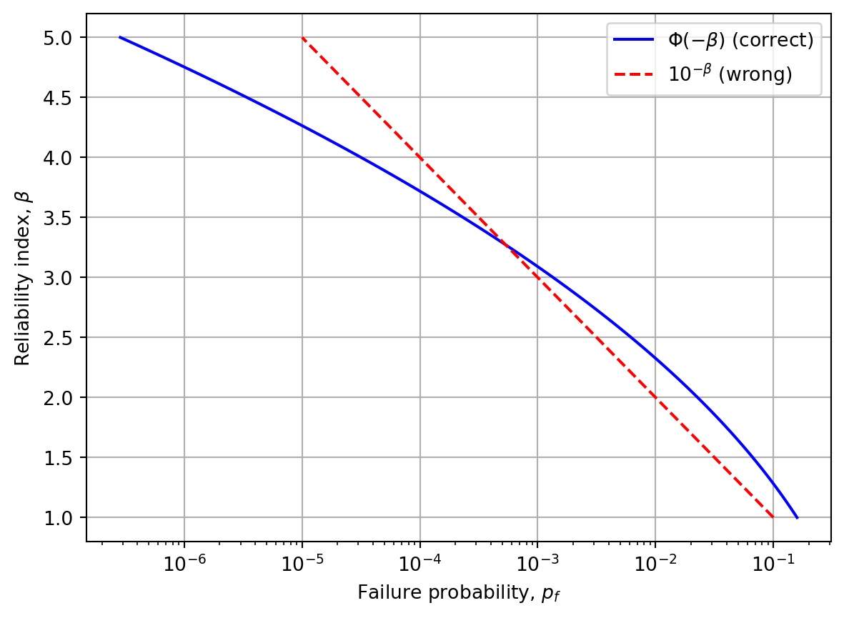
The fraction \(\frac{0 - \mu_g}{\sigma_g}\) in Equation 5.2 is necessary to ask a Standard Normal CDF for a probability, when the variable has mean \(\mu_g\) and standard deviation \(\sigma_g\). This is a probability transformation, explained in the next section. For now, we observe that the definition of the reliability index in Equation 5.1, first seen as the number of standard deviations from-mean-to-failure, is also justified as the argument in the calculation \(p_f = \Phi (-\beta)\).
The problem with the reliability index in Equation 5.1 is that it is only valid for linear limit-state functions. It gives different and contradictory results for equivalent nonlinear limit-state functions that should give the same result. Solving that problem, which is known from the 1970s literature as the invariance problem, is paramount in this book. That is because, as explained at the end of Chapter 1, all limit-state functions in structural analysis are nonlinear, regardless of whether the structural analysis is linear or nonlinear.
The solution to the invariance problem, first presented by Hasofer and Lind (1974), strengthens the interpretation of \(\beta\) as a distance from mean to failure, measured in terms of standard deviations. However, the solution relies on the transformation of the problem from the \(\mathbf{x}\) space of original variables to a \(\mathbf{y}\) space of Standard variables, each having zero mean and unit variance. The step from \(\mathbf{x}\) to \(\mathbf{y}\) represents a probability transformation, a topic addressed next.
5.2 Probability Transformation
The concept of probability transformations is, in a sense, the inverse of the problem addressed in Chapter 4. There, the objective was to determine the mean, \(\mu_u\), and standard deviation, \(\sigma_u\), for a known function, \(u(\mathbf{x})\). Conversely, the objective in the present section is to determine the function, for known mean and standard deviation.
To that end, we address a situation where \(\mu_x\), \(\sigma_x\), \(\mu_y\), and \(\sigma_y\) are all known. In fact, \(\mu_y=0\) and \(\sigma_y=1\) as implied by the label Standard used above. First considering the case of one random variable, the question is what the function \(y=h(x)\) is. Having the two values \(\mu_y=0\) and \(\sigma_y=1\) we try a linear function with two constants, \(a\) and \(b\):
\[ y = a + b \cdot x \tag{5.3}\]
Evaluating expectation integrals as in Chapter 4 yields expressions for \(\mu_y\) and \(\sigma_y\):
\[ \mu_y = \mathrm{E}[y] = \int_{-\infty}^{\infty} (a + b \cdot x) \cdot f(x) \,dx = a+b\cdot \mu_x \tag{5.4}\]
\[ \begin{aligned} \sigma_y^2 = \mathrm{E}[(y-\mu_y)^2] & = \int_{-\infty}^{\infty} (y-\mu_y)^2 \cdot f(x) \,dx = a+b\cdot \mu_x \\ &= \int_{-\infty}^{\infty} (y-\mu_y)^2 \cdot f(x) \,dx \\ &= \int_{-\infty}^{\infty} ((a + b \cdot x)-(a+b\cdot \mu_x))^2 \cdot f(x) \,dx \\ &= \int_{-\infty}^{\infty} (b \cdot x-b\cdot \mu_x)^2 \cdot f(x) \,dx \\ &= \int_{-\infty}^{\infty} (b^2 \cdot x^2 - 2 \cdot b^2 \cdot x \cdot \mu_x + b^2\cdot \mu_x^2) \cdot f(x) \,dx \\ &= b^2 \cdot \mathrm{E}[x^2] -2 \cdot b^2 \cdot \mathrm{E}[x] \cdot \mu_x + b^2\cdot \mu_x^2 \\ &= b^2 \cdot \left(\mathrm{E}[x^2] -\mu_x^2 \right) \\ &= b^2 \cdot \mathrm{Var}[x] \end{aligned} \tag{5.5}\]
The last equality employs the fact that the variance equals the mean square minus the square of the mean, which is derived as follows:
\[ \begin{aligned} \mathrm{Var}[x] &= \mathrm{E}[(x-\mu)^2] \\ & = \int_{-\infty}^{\infty} (x-\mu)^2 \cdot f(x) \,dx \\ & = \int_{-\infty}^{\infty} (x^2 -2\cdot \mu \cdot x + \mu^2) \cdot f(x) \,dx \\ &= \mathrm{E}[x^2] - 2 \cdot \mu \cdot \mathrm{E}[x] + \mu^2 \\ &= \mathrm{E}[x^2] - \mu^2 \end{aligned} \tag{5.6}\]
Setting \(\mu_y=0\) and \(\sigma_y=1\) and utilizing Equation 5.4 and Equation 5.5 gives \(a=-\frac{\mu_x}{\sigma_x}\) and \(b=\frac{1}{\sigma_x}\), which means the transformation in Equation 5.3 reads
\[ y = \frac{x - \mu_x}{\sigma_x} \Longleftrightarrow x = \mu_x + \sigma_x \cdot y \tag{5.7}\]
That is the transformation Cornell employed in Equation 5.2 to calculate \(p_f = \mathrm{P}(g<0)\) from a Standard Normal CDF for given \(\mu_g\) and \(\sigma_g\). The following subsection, and also Chapter 6, expands that simple probability transformation.
5.2.1 Correlation & Cholesky
Before we look at the solution to the invariance problem, potential correlation between the random variables should be accounted for. Specifically, we seek to extend the transformation in Equation 5.7 for non-zero off-diagonal components in the correlation and covariance matrices. In that case, the transformation must consider all random variables at once, instead of the one-by-one transformations implied by Equation 5.7. That means the candidate transformation in Equation 5.3 must be generalized to \(N\) linear functions of the \(N\) random variables:
\[ \mathbf{y} = \mathbf{a} + \mathbf{B} \mathbf{x} \tag{5.8}\]
where \(\mathbf{a}\) is a vector and \(\mathbf{B}\) is a matrix. Next, we calculate the mean of those functions, \(\pmb{\mu}_{\mathbf{y}}\), and the covariance matrix, \(\pmb{\Sigma}_{\mathbf{yy}}\) using properties of expectation employed earlier as well. Also, the fact that \(\mathbf{y}\) are Standard variables, i.e., having zero mean, unit variances, and zero correlation, gives the following two equations for the two unknowns \(\mathbf{a}\) and \(\mathbf{B}\):
\[ \pmb{\mu}_{\mathbf{y}} = \mathbf{a} + \mathbf{B} \pmb{\mu}_{\mathbf{x}} = \mathbf{0} \tag{5.9}\]
\[ \pmb{\Sigma}_{\mathbf{y}\mathbf{y}} = \mathbf{B} \pmb{\Sigma}_{\mathbf{xx}} \mathbf{B}^{\top} = \mathbf{I} \tag{5.10}\]
Pre-multiplying Equation 5.10 by \(\mathbf{B}^{-1}\) and also post-multiplying it by \(\mathbf{B}^{-\top}\) gives
\[ \pmb{\Sigma}_{\mathbf{xx}} = \mathbf{B}^{-1} \mathbf{B}^{-\top} \tag{5.11}\]
In words, \(\mathbf{B}\) is the matrix whose inverse, times its inverse transpose, equals the covariance matrix. That means \(\mathbf{B}^{-1}\) is the Cholesky decomposition of the covariance matrix. The Cholesky decomposition, which exists for square positive definite matrices, is a lower-triangular matrix that multiplied by the transpose of itself gives the original matrix. Of importance to the accuracy and stability of the Cholesky algorithm is that the components of the covariance matrix has units defined by the units of the random variables. That means the numerical values may vary significantly within the covariance matrix. This contrasts with the correlation matrix, whose components have values between \(-1\) and \(1\). This is why we prefer to rather decompose \(\mathbf{R}\), therefore rewriting Equation 5.11 using the definition in Equation 1.29 from Section 1.11:
\[ \pmb{\Sigma}_{\mathbf{xx}} = \mathbf{D}\mathbf{R}\mathbf{D} = \mathbf{D}\mathbf{L}\mathbf{L}^{\top}\mathbf{D} = \mathbf{B}^{-1} \mathbf{B}^{-\top} \tag{5.12}\]
where \(\mathbf{R} = \mathbf{L}\mathbf{L}^{\top}\) is the Cholesky decomposition. Substituting \(\mathbf{B}^{-1}=\mathbf{D}\mathbf{L}\), or rather
\[ \mathbf{B}=\mathbf{L}^{-1}\mathbf{D}^{-1} \tag{5.13}\]
into Equation 5.9 gives the other unknown: \[ \mathbf{a} = - \mathbf{L}^{-1}\mathbf{D}^{-1} \pmb{\mu}_{\mathbf{x}} \tag{5.14}\]
Substitution of Equation 5.13 and Equation 5.14 into Equation 5.8 gives the sought probability transformation that accounts for correlation:
\[ \mathbf{y} = \mathbf{L}^{-1}\mathbf{D}^{-1} \left( \mathbf{x} - \pmb{\mu} \right) \Longleftrightarrow \mathbf{x} = \pmb{\mu} + \mathbf{D}\mathbf{L} \mathbf{y} \tag{5.15}\]
It is reiterated that \(\pmb{\mu}\) contains the mean values for the random variables in \(\mathbf{x}\) and \(\mathbf{L}\) is the lower-triangular Cholesky decomposition of their correlation matrix, \(\mathbf{R}\). In the absence of correlation, \(\mathbf{L}\) is the identity matrix and Equation 5.15 simplifies to Equation 5.7. Both cases are considered in the following function, which will be amended in the next chapter, then making use of the distributions input that now is a placeholder:
def basicTransformation(y, means, stdvs, correlation, distributions):
    numRVs = len(means)
    if len(correlation) == 0:
        L = np.identity(numRVs)
    else:
        R = getR(means, correlation)
        L = np.linalg.cholesky(R)
    x = means + np.dot(np.dot(np.diag(stdvs), L), y)
    dxdy = np.dot(np.diag(stdvs), L)
    return x, dxdy
As often is the case in this book, error checks are omitted above for brevity. For example, checking the consistency of the input arrays would be prudent. The probability transformation in Listing 5.1 is employed in the reliability analyses coming in this chapter.
5.3 Solving the Invariance Problem
To solve the invariance problem, Hasofer and Lind (1974) transformed the reliability problem into the Standard \(\mathbf{y}\) space. Using Equation 5.7 or Equation 5.15, depending on the presence of correlation, \(\mathbf{y}\) is substituted for \(\mathbf{x}\) in the limit-state function. After doing so, it is customary to denote the limit-state function by the upper-case symbol \(G(\mathbf{y})\). It is instructive to take the step into the \(\mathbf{y}\) space for a linear limit-state function, here written
\[ g(\mathbf{x}) = a + \mathbf{b}^{\top} \mathbf{x} \tag{5.16}\]
where \(a\) and \(\mathbf{b}\) are constants different from those used earlier in this chapter. Substitution of Equation 5.15 for \(\mathbf{x}\) gives
\[ \begin{aligned} G(\mathbf{y}) &= a + \mathbf{b}^{\top} \left(\pmb{\mu} + \mathbf{D}\mathbf{L} \mathbf{y} \right) \\ &= \underbrace{a + \mathbf{b}^{\top}\pmb{\mu}}_{\equiv c} + \underbrace{\mathbf{b}^{\top}\mathbf{D}\mathbf{L}}_{\equiv \mathbf{d}^{\top}} \mathbf{y} \end{aligned} \tag{5.17}\]
Next, we calculate Cornell’s reliability index, defined in Equation 5.1, for the linear limit-state function in the Standard space, i.e., \(G(\mathbf{y}) = c + \mathbf{d}^{\top} \mathbf{y}\):
\[ \beta = \frac{\mu_G}{\sigma_G} = \frac{c}{\sqrt{\mathbf{d}^{\top}\mathbf{d}}} = \frac{c}{\lVert \mathbf{d} \rVert} \tag{5.18}\]
In that equation, \(\sigma_G\) is evaluated by recognizing that \(\nabla G=\mathbf{d}\) and that the covariance matrix of \(\mathbf{y}\) is the identity matrix. Interestingly, analytical geometry says that the smallest distance from the origin of a coordinate space, \(\mathbf{y}\), to the plane characterized by \(G(\mathbf{y})=0\) is exactly the result in Equation 5.18. From math books the formula for that distance is \(\Delta = \frac{G(\mathbf{0})}{\lVert \nabla G \rVert}\), which evaluates to \(\frac{c}{\lVert \mathbf{d} \rVert}\).
Because the means are zero and the standard deviations are unity in the \(\mathbf{y}\) space, the reliability index, \(\beta\), is the distance from the mean (origin) to failure (\(G=0\)), measured by number of standard deviations. Figure 5.1, described shortly, visualizes that point. However, it is valid only for linear limit-state functions. For nonlinear limit-state functions, which are omnipresent in structural reliability problems, Equation 5.1 is invalid. Nevertheless, the distance interpretation of \(\beta\) is helpful for addressing problems with nonlinear limit-state functions.
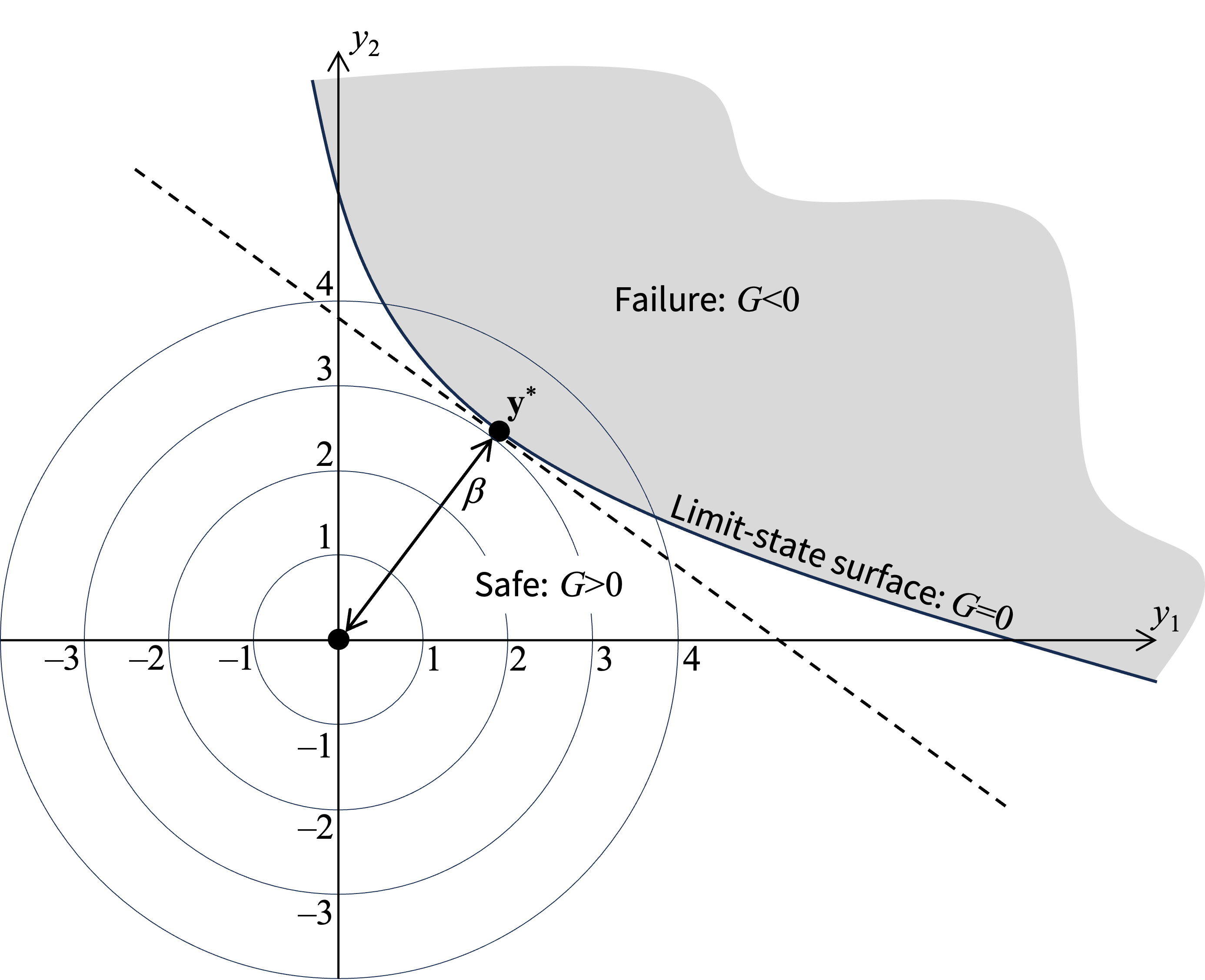
The Taylor linearization behind \(\mu_g\) and \(\sigma_g\) in Equation 5.1 gives the wrong reliability index because the linearization is made at the mean values of the random variables, i.e., the origin in the \(\mathbf{y}\) space. By consecutive linearization of the limit-state function, we can determine a better point for the linearization. Figure 5.1 illustrates this thinking. Linearization at the origin for nonlinear limit-state functions would not give the distance to the dashed line because of the approximation inherent in the Taylor linearization behind \(\mu_g\) and \(\sigma_g\). Rather, we must determine the location of the other solid black dot, which is a point on the limit-state surface that is shared by all equivalent limit-state functions, regardless of whether they are nonlinear.
This leads to the solution of the invariance problem. We perform an iterative search, described in the next section, for the point identified as \(\mathbf{y}^*\) in Figure 5.1, often referred to as the design point, and calculate the reliability index as the distance to that point:
\[ \beta = \lVert \mathbf{y}^* \rVert \tag{5.19}\]
That approach, based on a first-order approximation of the limit-state function at \(\mathbf{y}^*\), utilizing only second-moment information for the random variables, is abbreviated the FOSM method, i.e., first-order, second-moment.
This book argues that, in practical applications, valuable insights can be gained from omitting probability distributions. Basing reliability estimates on second-moment information, employing the reliability index as the primary result, is a transparent approach that often matches the available information. The reliability index is a proxy for the failure probability, and \(\beta\) is often specified explicitly in building codes and design standards. A target value of \(\beta\) between 3 and 4 are common in structural engineering. We observe a \(\beta\) value slightly above 3 in the schematic in Figure 5.1. For readers wishing to go beyond FOSM, the Chapter 6 is offered.
5.4 HLRF Algorithm
As alluded to above, reliability analysis with nonlinear limit-state functions requires an iterative search for the point \(\mathbf{y}^*\), which is needed for the determination of the reliability index \(\beta\). \(\mathbf{y}^*\) is the solution to the equality-constrained optimization problem
\[ \mathbf{y}^* = \mathrm{argmin}(\lVert \mathbf{y} \rVert \; | \; G(\mathbf{y})=0) \tag{5.20}\]
In words, we seek the point on the boundary between the failure domain and the safe domain, i.e., \(G(\mathbf{y})=0\) that has the minimum distance to the origin in the \(\mathbf{y}\) space. An equivalent version of Equation 5.20, valid when the mean realization of the input variables represents a safe structure, i.e., \(G(\mathbf{0})>0\), is
\[ \mathbf{y}^* = \mathrm{argmin}(\frac{1}{2} \lVert \mathbf{y} \rVert^2 \; | \; G(\mathbf{y})<0) \tag{5.21}\]
That formulation is addressed by a larger class of generic optimization algorithms. To solve Equation 5.20, the algorithm known as Hasofer-Lind-Rackwitz-Fiessler repeatedly generates trial points, \(\mathbf{y}_{(m)}\), until convergence at \(\mathbf{y}^*\), with \(m\) serving as iteration counter starting at \(m=1\). Parentheses in the subscript are employed to highlight that \(\mathbf{y}_{(m)}\) is vector number \(m\), not the \(m^{\text{th}}\) entry in the vector. The derivation of the recursive HLRF algorithm starts with the Taylor linearization of the limit-state function at \(\mathbf{y}_{(m)}\):
\[ \bar{G}_m \approx G(\mathbf{y}_{(m)}) + \nabla G_m^{\top} (\mathbf{y}-\mathbf{y}_{(m)}) \tag{5.22}\]
As mentioned earlier, according to analytical geometry the smallest distance from the origin in the standard space, \(\mathbf{y}=\mathbf{0}\), to the plane where \(\bar{G}_m=0\) is
\[ \Delta_m = \frac{\bar{G}_m(\mathbf{0})}{\lVert \nabla \bar{G}_m \rVert} = \frac{G(\mathbf{y}_{(m)}) - \nabla G_m^{\top} \mathbf{y}_{(m)}}{\lVert \nabla G_m \rVert} = \frac{G(\mathbf{y}_{(m)})}{\lVert \nabla G_m \rVert} + \pmb{\alpha}_{(m)}^{\top} \mathbf{y}_{(m)} \tag{5.23}\]
The \(\pmb{\alpha}\) vector is introduced in the last equality. Well known in the reliability literature, it is a unit-length vector defined as the negative normalized gradient vector:
\[ \pmb{\alpha} = -\frac{\nabla G}{\lVert \nabla G \rVert} \tag{5.24}\]
Figure 5.2 visualizes both \(\Delta_m\) and \(\pmb{\alpha}_{(m)}\) to aid the understanding of the recursive HLRF algorithm, which reads
\[ \mathbf{y}_{(m+1)} = \Delta_m \cdot \pmb{\alpha}_{(m)} \tag{5.25}\]
To follow a few steps with that algorithm, notice first in Figure 5.2 that the \(\pmb{\alpha}\) vectors point away from the origin. That is because the origin is in the safe region, where \(G>0\). The gradient vector \(\nabla G\) points in the direction of increasing \(G\)-function value; thus, \(\pmb{\alpha}\) points in the opposite direction, away from the origin.
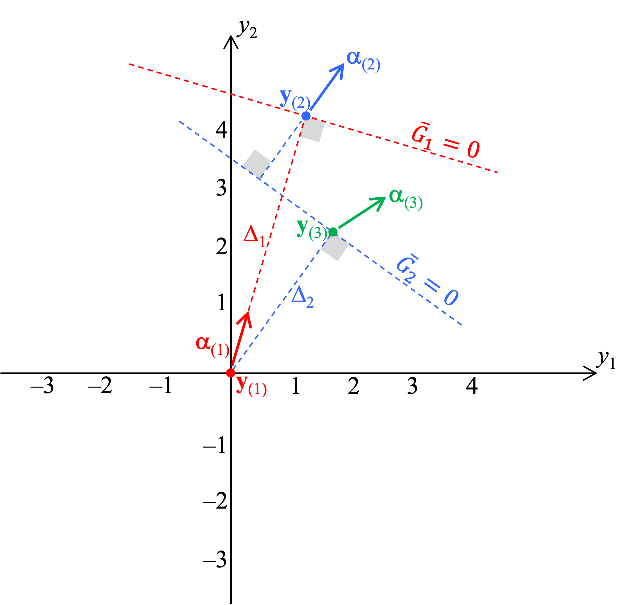
Next, consider the T-shape formed by the red dashed lines in Figure 5.2. The orientation of that T is determined by the vector \(\pmb{\alpha}_{(1)}\) calculated at the first trial point, \(\mathbf{y}_{(1)}\). From that point, a red dashed lines emanates, following the direction of the \(\pmb{\alpha}\) vector until it hits the line where the linearized limit-state function, \(\bar{G}_1\), is zero. If the original limit-state function had been linear, then the blue dot, i.e., \(\mathbf{y}_{(2)}\) would have been the sought design point, \(\mathbf{y}^*\) and \(\Delta_1\) would be the sought reliability index. However, because the limit-state function is nonlinear, the red dashed line in Figure 5.2 that marks \(\bar{G}_1=0\) is not where \(G=0\), and the algorithm continues from the new trial point \(\mathbf{y}_{(2)}=\Delta_1 \pmb{\alpha}_{(1)}\).
At the second trial point, \(\mathbf{y}_{(2)}\), the \(\pmb{\alpha}\) vector is recalculated. The result, \(\pmb{\alpha}_{(2)}\), determines the orientation of the blue dashed lines in Figure 5.2. The blue dashed line that emanates from \(\mathbf{y}_{(2)}\) reaches the perpendicular line where the linearized limit-state function is zero, \(\bar{G}_2=0\). The point on that line that is closest to the origin is the new trial point, \(\mathbf{y}_{(3)} = \Delta_2 \cdot \mathbf{y}_{(2)}\). It is marked with a green dot in Figure 5.2, and the new \(\pmb{\alpha}\) vector, \(\pmb{\alpha}_{(3)}\), is calculated at that location. It is now time to check convergence, which consists of two criteria:
The original limit-state function evaluated at the trial point must be close to zero: \(G(\mathbf{y}_{(m)}) \approx 0\). One way to check that, is to require that \(\left| \frac{G(\mathbf{y}_{(m)})}{G(\mathbf{y}_{(1)})}\right| < 10^{-2}\), where \(G(\mathbf{y}_{(1)})\) is the value of the limit-state function at the first trial point, serving as normalizing constant
The gradient vector evaluated at the trial point must point at the origin. One way to check that, is to require that \(1 - \mathrm{cos}(\theta) = 1 - \pmb{\alpha}_{(m)}^{\top}\frac{\mathbf{y}_{(m)}}{\lVert \mathbf{y}_{(m)} \rVert} < 10^{-2}\), where \(\theta\) is the angle between the \(\pmb{\alpha}\) vector and the line from the origin to the trial point
In Figure 5.2 we observe that the green arrow representing \(\pmb{\alpha}_{(3)}\) does not align with the origin. In other words, \(\pmb{\alpha}_{(3)}\) and \(\mathbf{y}_{(3)}\) are not parallel vectors; hence, the search for \(\mathbf{y}^*\) would need to continue, repeating the steps described above.
5.5 Evaluating \(G\) and \(\nabla G\)
In the input to a structural reliability analysis, the limit-state function is specified in the original \(\mathbf{x}\) space of random variables. An example is Equation 1.19. Conversely, the search for the design point described above, which ultimately gives the reliability index via Equation 5.19, takes place in the \(\mathbf{y}\) space. In this situation, \(G\) and \(\nabla G\) are evaluated as follows, at every step of the HLRF algorithm:
The trial point \(\mathbf{y}_{(m)}\) is determined from Equation 5.25
The trial point is transformed into the original variable space by the right-most formula in Equation 5.15
Now having \(\mathbf{x}_{(m)}\), i.e., the input values to the structural analysis, the structural analysis is run to obtain \(u(\mathbf{x}_{(m)})\) and \(\frac{\partial u(\mathbf{x}_{(m)})}{\partial \mathbf{x}}\)
The value of the limit-state function for the example in Equation 1.19 is identical to the value in the Standard space: \(g(\mathbf{x}_{(m)}) = G(\mathbf{y}_{(m)})\)
The gradient vector in the \(\mathbf{y}\) space, required in Equation 5.23 and Equation 5.24, is calculated by the chain rule of differentiation: \(\nabla G = \frac{\partial G}{\partial \mathbf{y}} = \frac{\partial g}{\partial u}\frac{\partial u}{\partial \mathbf{x}}\frac{\partial \mathbf{x}}{\partial \mathbf{y}}\), where \(\frac{\partial g}{\partial u}=-1\) because of Equation 1.19, \(\frac{\partial u}{\partial \mathbf{x}}\) is provided by the structural analysis, and \(\frac{\partial \mathbf{x}}{\partial \mathbf{y}}=\mathbf{DL}\) from the right-most formula in Equation 5.15
5.6 Line Search for Optimal Step Size
The recursive algorithm expressed in Equation 5.25 is a gradient-based optimization algorithm addressing Equation 5.20. Applied to limit-state functions that are highly nonlinear in the \(\mathbf{y}\) space, sometimes due to probability transformations accounting for full distributions, the HLRF algorithm may struggle. Work led by Professor Der Kiureghian at UC Berkeley linked the HLRF algorithm with techniques developed in the more general field of optimization. To that end, Equation 5.25 is rewritten as \[ \mathbf{y}_{(m+1)} = \mathbf{y}_{(m)} + s_m \cdot \mathbf{d}_{(m)} \tag{5.26}\]
where \(s=\) step size and \(\mathbf{d}=\) search direction defined as
\[ \begin{aligned} \mathbf{d}_{(m)} &= \mathbf{y}_{(m+1)} - \mathbf{y}_{(m)} \\ &= \Delta_m \cdot \pmb{\alpha}_{(m)} - \mathbf{y}_{(m)} \end{aligned} \tag{5.27}\]
That last equation represents a merger between Equation 5.26 with Equation 5.23 and Equation 5.25. A visual example of a search direction vector is the imaginary line that connects \(\mathbf{y}_{(2)}\) and \(\mathbf{y}_{(3)}\) in Figure 5.2.
It is the introduction of a step size, \(s_m\), determined by a line search along the direction \(\mathbf{d}_{(m)}\), that justifies the prefix “i” in the improved iHLRF algorithm coined by Der Kiureghian (2022). The default value implied by Equation 5.25 is \(s_m=1\). However, for challenging problems this causes convergence problems. Such problems mimic those sometimes seen in the application of the basic Newton algorithm for root-finding. In the following, a line search along \(\mathbf{d}_{(m)}\) is conducted to find the step size that minimizes a merit function, here expressed as
\[ \begin{aligned} m(s) &= a \cdot \lVert \mathbf{y}(s) \rVert + b \cdot \left| \frac{G(\mathbf{y}(s))}{G(\mathbf{y}_{(1)})} \right| \end{aligned} \tag{5.28}\]
where Equation 5.26 gives \(\mathbf{y}(s) = \mathbf{y}_{(m)} + s \cdot \mathbf{d}_{(m)}\) and \(a\) and \(b\) are constants different from those defined earlier in this chapter. Different choices for \(a\) and \(b\) weigh \(\lVert \mathbf{y} \rVert\) and \(G\) differently. Without getting into details of optimization theory, \(a=1\) and \(b=5\) are employed in the code presented below.
Several 1D optimization algorithms are available for the search for an optimal step size. The Armijo rule, repeatedly halving or otherwise reducing the step size from unity is one option. Instead, the golden section algorithm is employed here. Illustrated in Figure 5.3, it is an algorithm based on the golden section ratio, which also appears in aesthetical studies.
At every iteration, this algorithm employs the value of the merit function at three candidate step sizes. At first, assume we have evaluated the merit function at the points \(s_1\), \(s_2\), and \(s_3\) identified in Figure 5.3. Because \(m(s_2)\) is less than the value at its closest neighbour \(s_1\), the optimal solution must lie in the longer interval, from \(s_2\) to \(s_3\). That is why the new trial step size, \(s_4\), marked with red in Figure 5.3 is placed in that interval, closest to \(s_2\).
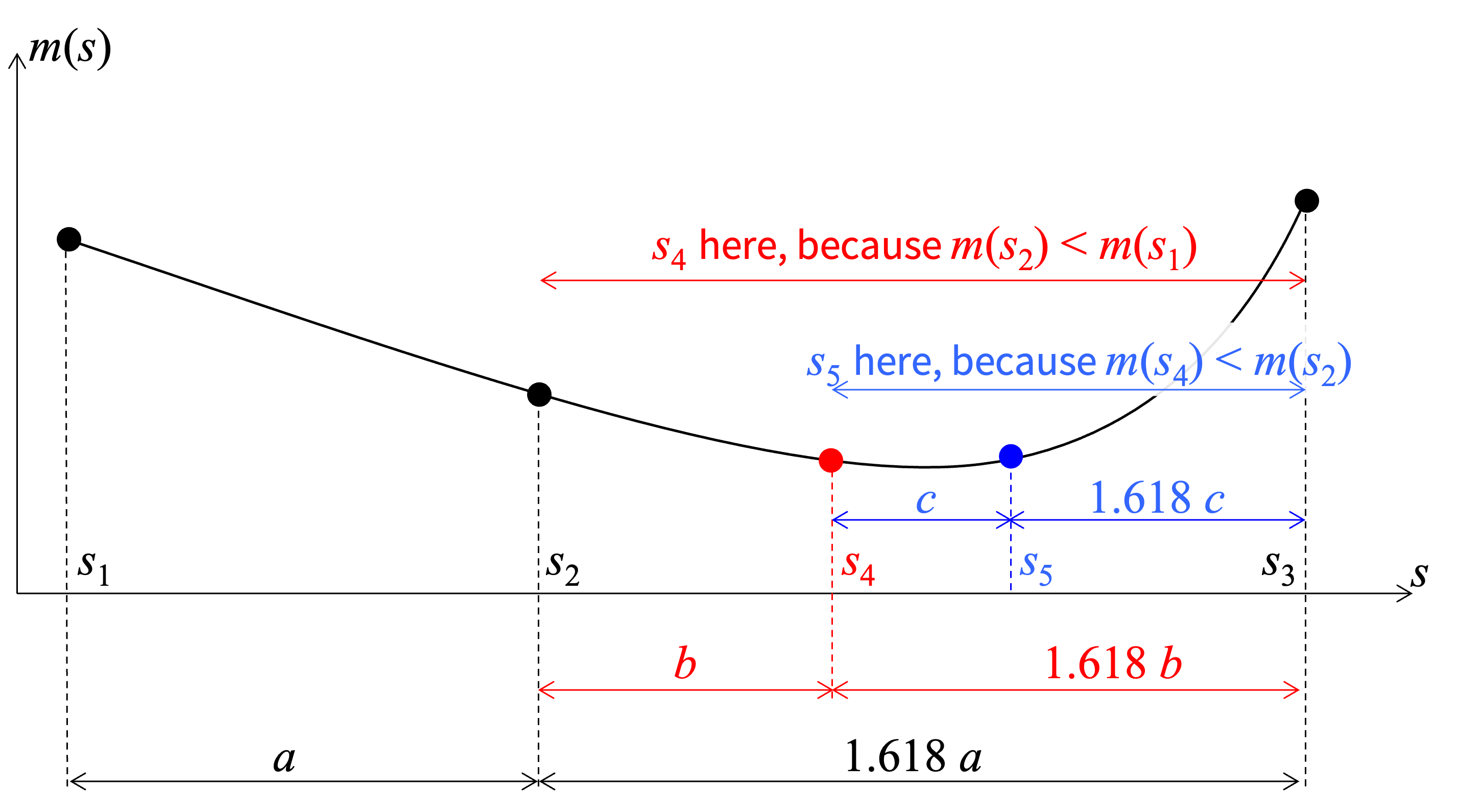
Next, after evaluating \(m(s_4)\) and finding that the value is smaller than the value at its closest neighbour, \(s_2\), the conclusion is drawn that the optimum solution must lie in the longer interval, from \(s_4\) to \(s_3\). That is why the new trial step size, \(s_5\), marked with blue in Figure 5.3 is placed in that interval, closest to \(s_4\). The golden section search algorithm is implemented in the following function:
def goldenSectionLineSearch(F, lowerBound, upperBound, printProgress=True):
    goldenRatio = (1.0 + np.sqrt(5.0)) / 2.0
    x1 = lowerBound
    x4 = upperBound
    theRange = x4 - x1
    bigPortionOfRange = theRange / goldenRatio
    x2 = x4 - bigPortionOfRange
    x3 = x1 + bigPortionOfRange
    Fx1 = F(x1)
    Fx2 = F(x2)
    Fx3 = F(x3)
    Fx4 = F(x4)
    convergence = False
    counter = 0
    while not convergence:
        counter += 1
        if Fx3 > Fx2:
            theRange = x3 - x1
            bigPortionOfRange = theRange / goldenRatio
            x4 = x3
            Fx4 = Fx3
            x3 = x2
            Fx3 = Fx2
            x2 = x4 - bigPortionOfRange
            Fx2 = F(x2)
        else:
            theRange = x4 - x2
            bigPortionOfRange = theRange / goldenRatio
            x1 = x2
            Fx1 = Fx2
            x2 = x3
            Fx2 = Fx3
            x3 = x1 + bigPortionOfRange
            Fx3 = F(x3)
        if np.abs(x3 - x2) < 0.01:
            optimum = (x2 + x3) / 2.0
            convergence = True
    if printProgress:
        print(f"Line search converged to s={optimum:.2f} after {counter} iterations")
    return optimum
5.7 Reliability Analysis
The improved HLRF algorithm, with the golden section search for optimal step sizes, is now implemented and tested. The algorithm takes a limit-state function as input, as well as a response threshold employed by that function. Second-moment information for the random variables is also given as input, together with the probability transformation, which will be amended in the next chapter.
That last two optional inputs are the lineSearchFlag, which can be set to False to circumvent the golden section search in favour of \(s_m=1\), reducing the number of evaluations of the limit-state function, and a print flag to avoid excessive output when the algorithm is run sequentially for several response thresholds:
def iHLRFalgorithm(g, threshold, means, stdvs, correlation, distributions, transformation, lineSearchFlag=True, printProgress=True):
    numRVs = len(means)
    y = np.zeros(numRVs)
    maxNumTrials = 50
    for i in range(1, maxNumTrials):
        x, dxdy = transformation(y, means, stdvs, correlation, distributions)
        gValue, dgdx = g(x, threshold)
        dGdy = dgdx.dot(dxdy)
        gradientNorm = np.linalg.norm(dGdy)
        alpha = np.multiply(dGdy, -1 / gradientNorm)
        yNorm = np.linalg.norm(y)
        if i == 1:
            gfirst = gValue
            yNorm = 1
        criterion1 = np.abs(gValue / gfirst)
        yScaled = np.multiply(y, 1.0/yNorm)
        yScaledAlpha = yScaled.dot(alpha)
        criterion2 = np.linalg.norm(np.subtract(yScaled, np.multiply(alpha, yScaledAlpha)))
        if printProgress:
            print(f"HLRF step {i}: Check1={criterion1:.2e},Check2={criterion2:.2e}, y-norm={yNorm:.3f}")
        if criterion1 < 1e-2 and criterion2 < 1e-2:
            beta = np.linalg.norm(y) * np.sign(gfirst)
            if np.array_equal(alpha, previousAlpha):
                kappa = 0
            else:
                kappa = np.arccos(alpha.dot(previousAlpha)) / np.sqrt(np.linalg.norm(y-previous_y)**2 - np.linalg.norm(alpha.dot(y-previous_y))**2)
            if printProgress:
                print(f"iHLRF algorithm converged with beta={beta:.3f}")
            return beta, x, y, kappa
        else:
            if i == 49:
                print("ERROR: iHLRF algorithm did not converge.")
                return 0, 0, 0, 0
            previous_y = np.copy(y)
            previousAlpha = np.copy(alpha)
            searchDirection = np.multiply(alpha, (gValue / gradientNorm + alpha.dot(y))) - y
            def meritFunction(stepSize):
                yTrial = y + stepSize * searchDirection
                yNormTrial = np.linalg.norm(yTrial)
                xTrial, void = transformation(yTrial, means, stdvs, correlation, distributions)
                gTrial, void = g(xTrial, threshold, False)
                return yNormTrial + 5 * np.abs(gTrial/gfirst)
            if lineSearchFlag:
                stepSize = goldenSectionLineSearch(meritFunction, 0, 1.5, printProgress)
            else:
                stepSize = 1.0
            y += stepSize * searchDirection
As usual, it would not hurt to add a few error checks to that code. For example, checking that the second-moment arrays have consistent shapes would be good. The limit-state function below asks for the probability that the horizontal displacement at the top left corner of the frame exceeds the value given by threshold:
def linearFrameLSF(x, threshold, needGradient=True):
    void, void, void, void, trackNode, trackDOF, DDMs = linearFrameVariableSpecs()
    input = createLinearFrameInput(*x)
    structuralModel = model(input)
    if needGradient:
        u, dudx = linearStaticFirstOrder(structuralModel, trackNode, trackDOF, DDMs)
    else:
        u = linearStaticResponse(structuralModel, trackNode, trackDOF)
        dudx = 0
    return (threshold-u), -dudx
Notice that -dudx is returned because of the explanations in Section 5.5. Next, the iHLRF algorithm is tested for the portal frame, asking for the reliability index associated with the response exceeding 25mm:
means, stdvs, distributions, correlation, trackNode, trackDOF, DDMs = linearFrameVariableSpecs()
beta, xStar, yStar, kappa = iHLRFalgorithm(linearFrameLSF, 0.025, means, stdvs, correlation, distributions, basicTransformation)
HLRF step 1: Check1=1.00e+00,Check2=0.00e+00, y-norm=1.000
Line search converged to s=0.88 after 8 iterations
HLRF step 2: Check1=9.84e-03,Check2=1.76e-01, y-norm=2.074
Line search converged to s=1.01 after 8 iterations
HLRF step 3: Check1=6.51e-05,Check2=8.33e-03, y-norm=2.060
iHLRF algorithm converged with beta=2.060We observe in the output that only three steps of the iHLRF algorithm are needed to determine the reliability index, and that the optimal step size is consistently quite close to unity. This implies that the golden section line search might not be necessary for the present case. Evaluations of the limit-state functions are saved by skipping that line search. Therefore, it is here attempted to run the same reliability analysis with a unit step size:
beta, xStar, yStar, kappa = iHLRFalgorithm(linearFrameLSF, 0.025, means, stdvs, correlation, distributions, basicTransformation, False)HLRF step 1: Check1=1.00e+00,Check2=0.00e+00, y-norm=1.000
HLRF step 2: Check1=1.46e-01,Check2=1.99e-01, y-norm=2.359
HLRF step 3: Check1=3.28e-03,Check2=2.73e-02, y-norm=2.055
HLRF step 4: Check1=2.84e-05,Check2=1.46e-03, y-norm=2.060
iHLRF algorithm converged with beta=2.060That was successful; although one more iHLRF iteration was needed, many evaluations of the limit-state function, i.e., structural analyses were avoided.
Insights can be gained by observing the random variable realizations that are the most likely to cause failure, i.e., to cause the displacement to reach the threshold. Here are the \(\mathbf{x}\) values at the design point:
names = ['E', 'A', 'I', 'q', 'F']
for i in range(len(xStar)):
    print(f"{names[i]} is now {xStar[i]:.2e} versus mean value {means[i]:.2e}")
E is now 1.75e+11 versus mean value 2.00e+11
A is now 1.88e-02 versus mean value 1.88e-02
I is now 4.49e-04 versus mean value 4.62e-04
q is now 2.59e+04 versus mean value 2.00e+04
F is now 6.46e+04 versus mean value 5.00e+04We naturally observe that the loads \(F\) and \(q\) are higher at failure, while \(E\) and \(I\) are lower. Moreover, we see once more that the cross-section area is not an important variable for this portal frame.
5.8 Sampling
Similar to the ending of the previous chapter, the more computationally costly sampling approach, referred to as Monte Carlo sampling, is implemented here. The objective is to compare the \(\beta\) value from FOSM with that obtained by sampling. To do so, it is necessary to assume the Normal distribution for the random variables in the sampling algorithm. Additionally, it is necessary to solve Equation 5.2 for \(\beta\) after the sampling is done. Notice that \(p_f\) is the number of failures divided by the total number of samples:
def samplingAlgorithm(g, threshold, means, stdvs, correlation, numSamples):
    numRVs = len(means)
    if len(correlation) > 0:
        R = getR(means, correlation)
        L = np.linalg.cholesky(R)
    else:
        L = np.identity(numRVs)
    y = np.zeros(numRVs)
    failureCount = 0
    for i in range(numSamples):
        y = np.random.normal(0, 1, numRVs)
        x = means + np.dot(np.dot(np.diag(stdvs), L), y)
        gValue, void = g(x, threshold, False)
        if gValue < 0:
            failureCount += 1
    if failureCount == 0:
        print("No failures encountered in sampling analysis")
    else:
        pf = failureCount/numSamples
        beta = -norm.ppf(pf)
        print(f"beta from sampling: {beta:.3f}")
Depending on the distance from the origin to the limit-state surface in the \(\mathbf{y}\) space and the number of samples generated, the Monte Carlo result may be a rough approximation. That is why it would be meaningful to repeat the following sampling analysis with more samples and different seeds for the random number generator:
numSamples = int(1e5)
samplingAlgorithm(linearFrameLSF, 0.025, means, stdvs, correlation, numSamples)
beta from sampling: 2.0555.9 Reliability Index vs. Standard Deviation
Earlier it is established that the reliability index, \(\beta\), is the number of standard deviations from the mean to the closest point in the failure region. That statement is valid in the \(\mathbf{y}\) space. Now consider a situation where failure is defined as the response exceeding the threshold \(\mu_u + c \cdot \sigma_u\), where \(\mu_u\) and \(\sigma_u\) are response statistics calculated in the previous chapter. That means \(c\) is the number of first-order approximate standard deviations from the second-order approximate mean. The plot below compares \(c\) with \(\beta\) for different values of \(c\):
covarianceMatrix = getCovMatrix(means, stdvs, correlation)
input = createLinearFrameInput(*means)
structuralModel = model(input)
u, dudx, Hessian = linearStaticSecondOrder(structuralModel, trackNode, trackDOF, DDMs)
meanSO = u + 0.5 * np.sum(Hessian * covarianceMatrix)
stdvFO = np.sqrt(dudx.dot(covarianceMatrix.dot(dudx)))
plt.figure()
for c in np.linspace(1, 4, 20):
    threshold = meanSO + c * stdvFO
    beta, xStar, yStar, kappa = iHLRFalgorithm(linearFrameLSF, threshold, means, stdvs, correlation, distributions, basicTransformation, True, False)
    plt.plot(c, beta, 'ko', markersize=3)
plt.xlabel("$c$")
plt.ylabel("$\\beta$")
plt.axline((1, 1), slope=1, color='black', linestyle='--')
plt.grid(True)
plt.show()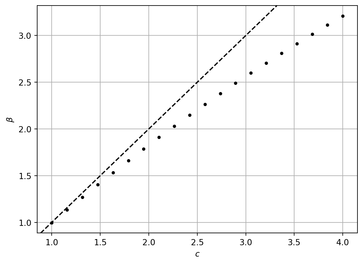
Along the dashed line, \(c=\beta\). We observe a mismatch between \(c\) and \(\beta\) that increases with the distance from mean to failure. For example, the idea that exceeding “mean response plus \(3\) response standard deviations,” using second-moment approximations, corresponds to \(\beta=3\) is erroneous and unconservative. The plot above suggests a reliability index consistently below the corresponding number of standard deviations from the mean response.