from Chapter9code import *10 Linear Dynamics
Structural dynamics is a large and interesting field of study, certainly relevant in earthquake engineering. The objective in this chapter is to establish the governing response equations, solving them with a time-stepping algorithm, while simultaneously calculating response sensitivities. The concept of pseudo time, introduced in Chapter 8, here transitions to real time.
10.1 Equation of Motion
Multi-DOF analysis is the goal of this chapter. However, developing solutions for single-DOF problems is an important part of structural dynamics, for several reasons. One is that linear multi-DOF problems can be decoupled into single-DOF problems in what is known as modal analysis. Another reason is the insights gained from analytical solutions for single-DOF problems, for various loading scenarios and even free vibration. However, this book emphasizes computational methods. The equilibrium equation for a single-DOF system is established here as a stepping stone towards solving multi-DOF problems.
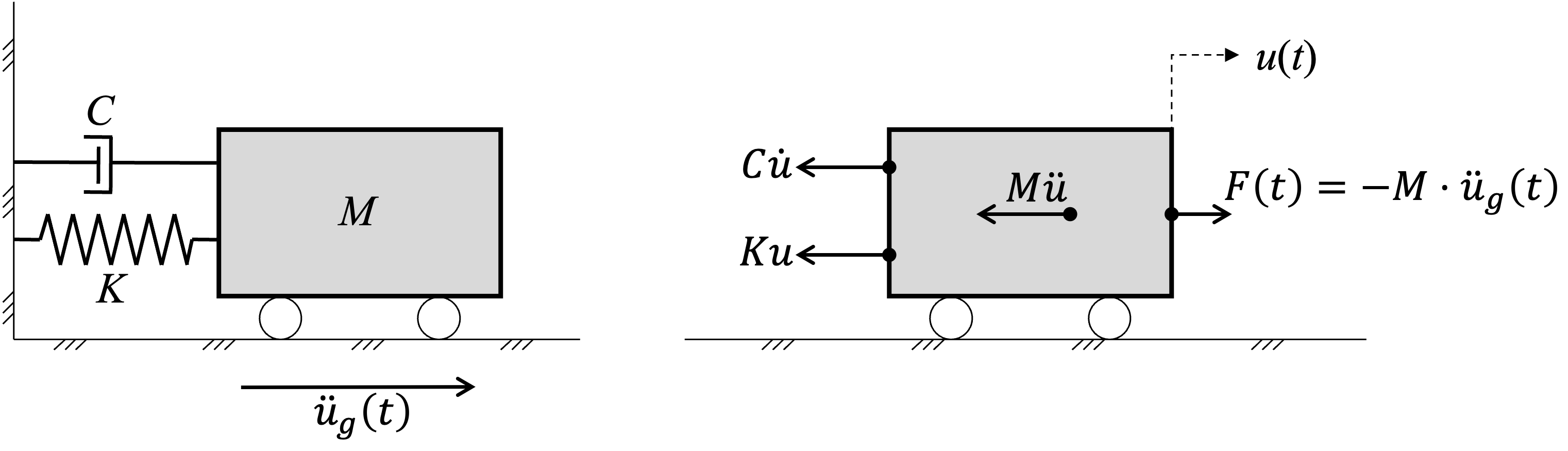
The left-hand side of Figure 10.1 shows a grey-shaded mass, freely rolling in the horizontal direction, except being held back by a spring with stiffness \(K\) and a dashpot with damping constant \(C\). Notice the cause of the external force imparted on the mass; the ground is accelerating, denoted by \(\ddot{u}_g(t)\). Each dot above a symbol means one derivative with respect to time. The right-hand side of Figure 10.1 highlights the forces acting upon the mass, including that from the ground motion:
- The effect of the ground accelerating towards the right is according to Newton’s second law an external force applied towards the left, hence the minus sign in Figure 10.1, equal to mass times acceleration, i.e., \(M \cdot \ddot{u}_g(t)\)
- The effect of the mass itself accelerating towards the right is from d’Alembert applying Newton’s law an inertia force equal to mass times acceleration, \(M \cdot \ddot{u}\), towards the left
- The effect of the mass having a velocity towards the right is a viscous force from the dashpot equal to \(C \cdot \dot{u}\) towards the left
- The effect of the mass displacing towards the right is an elastic force from the spring equal to \(K \cdot u\) towards the left
Notice that \(u\) is the relative displacement of the mass, relative to the moving ground. That means \(\dot{u}\) and \(\ddot{u}\) are also measured relative to the ground. However, the role of the total acceleration, \(\ddot{u} + \ddot{u}_g\), is important in earthquake engineering, as explained shortly.
Equilibrium of the mass shown in the right-hand side of Figure 10.1 gives
\[ M\cdot \ddot{u} + C \cdot \dot{u} + K \cdot u = -M \cdot \ddot{u}_g(t) \tag{10.1}\]
10.2 Natural Frequency
Equation 10.1 is a second-order differential equation with constant coefficients, referred to as the equation of motion. If we consider free undamped vibration, i.e., neglecting the right-hand side and the damping term, its solution is
\[ u(t) = A \cdot \mathrm{cos}(\omega_n \cdot t) + B \cdot \mathrm{sin}(\omega_n \cdot t) \tag{10.2}\]
where
\[ \omega_n = \sqrt{\frac{K}{M}} \tag{10.3}\]
is called the natural frequency of vibration. It is an important physical characteristic that reveals the excitation frequency, in radians per second, that the system is most vulnerable to. It is expressed equivalently as the natural period of vibration, in seconds:
\[ T_n = \frac{2 \pi}{\omega_n} \tag{10.4}\]
10.3 Role of Total Acceleration
Later in this chapter, eigenvalue analysis will reveal a number of natural periods for multi-DOF structures matching the number of DOFs with mass in the structural model. Consider such a structure, specifically a high-rise building. When subjected to ground motion, it is bound to respond primarily in one displaced shape; the one with steadily increasing displacement from the base to the roof. Suppose that displaced shape is associated with the natural period of vibration \(T_n\). Then we can think of that structure as a single-DOF problem with that natural period.
Next, we imagine analyzing that SDOF problem with a time-stepping algorithm, such as the one presented later in this chapter. In earthquake engineering, it is common to use the total, not relative acceleration response from that analysis to find the base shear force that the building must be designed for. To understand why the total acceleration response is correct, we revisit the force \(K \cdot u\) in the spring in Figure 10.1:
\[ F = K \cdot u = M \cdot \omega_n^2 \cdot u \tag{10.5}\]
where Equation 10.3 is utilized in the last equality. Let us keep Equation 10.5 in mind as we proceed to rearrange the free undamped version of Equation 10.1 into the form
\[ \ddot{u} + \ddot{u}_g = -\frac{K}{M} \cdot u = - \omega_n^2 \cdot u \tag{10.6}\]
where Equation 10.3 is utilized again in the last equality. Combining Equation 10.5 and Equation 10.6 gives
\[ F = - M \cdot \left( \ddot{u} + \ddot{u}_g \right) \tag{10.7}\]
thus explaining why it is correct to multiply the mass by the total acceleration to obtain the force. By running the analysis for many \(T_n\) values and plotting the maximum value of \(\ddot{u}(t)+\ddot{u}_g(t)\) during the shaking along the \(T_n\) axis, we form what are called the acceleration response spectrum, \(S_a(T_n)\).
By doing that for many ground motions, and applying techniques from statistics, building codes provide “design spectra” for \(S_a(T_n)\), which engineers employ to determine the earthquake force on structures. Notice that Equation 10.6 says that one can obtain the same result, with a small approximation for large damping values, by using the “pseudo response spectrum” \(S_a(T_n) \approx \omega_n^2 \cdot \mathrm{max}\left(u(t) \right)\).
10.4 Lumped Mass Matrix
The objective is now to generalize Equation 10.1 to multi-DOF problems. A sense of the end result was provided in Equation 1.5, and the first term in that equation, i.e., the inertia term with a mass matrix, is addressed first. The derivation can be done the easy way, or the hard way. The harder approach is to establish dynamic equilibrium for an infinitesimally short beam element, use that to set up the differential equation with elastic and inertia forces, derive the “weak form” of that boundary value problem, representing the principle of virtual displacements, and use the shape functions of the finite element method to establish the mass matrix and the stiffness matrix.
That is a powerful approach that gives a mass matrix with off-diagonal terms that include the effect of distributed mass along each frame element. However, in practical applications it is more common to “lump” all mass onto selected DOFs. That is done in the following example, which is a vertical cantilevered column divided into nel linear frame elements. Notice how the mass is concentrated along the horizontal DOF at every node along the column, the top node having half that of the others because it has only one adjacent element:
def createLinearColumnInput(E, A, I, rho, nel):
    L = 10
    M = A * L/nel * rho
    q = 0
    NODES = []
    for i in range(nel+1):
        NODES.append([0.0, i*L/nel])
    CONSTRAINTS = [[1, 1, 1]]
    for i in range(nel):
        CONSTRAINTS.append([0, 0, 0])
    ELEMENTS = []
    for i in range(nel):
        ELEMENTS.append([5, E, A, I, q, i+1, i+2])
    SECTIONS = np.zeros(nel)
    MATERIALS = np.zeros(nel)
    LOADS = np.zeros((nel+1, 3))
    MASS = [[0, 0, 0]]
    for i in range(nel-1):
        MASS.append([M, 0, 0])
    MASS.append([0.5*M, 0, 0])
    input = [NODES, CONSTRAINTS, ELEMENTS, SECTIONS, MATERIALS, LOADS, MASS]
    return input
The following function, added to the structural model class, provides the derivative of the mass matrix, given input shown near the end of this chapter:
class model(model):
    def getMassDerivative(self, dMin):
        nnodes = np.size(self.DOF, 0)
        numdofnod = np.size(self.DOF, 1)
        ntot = nnodes * numdofnod
        dM = np.zeros(ntot)
        if np.size(dMin, 1) > 0:
            for i in range(nnodes):
                id = self.DOF[i,:]
                dM[id] = dM[id] + dMin[i][:]
        dM = np.diag(dM)
        return dM
Here is a plot of the structure defined above:
E = 200e9         # N/m^2
A = 18774e-6      # m^2 (W360X147 = W14x99)
I = 462016882e-12 # m^4
rho = 7850.0      # kg/m^3
nel = 5
input = createLinearColumnInput(E, A, I, rho, nel)
structuralModel = model(input)
structuralModel.plotModel()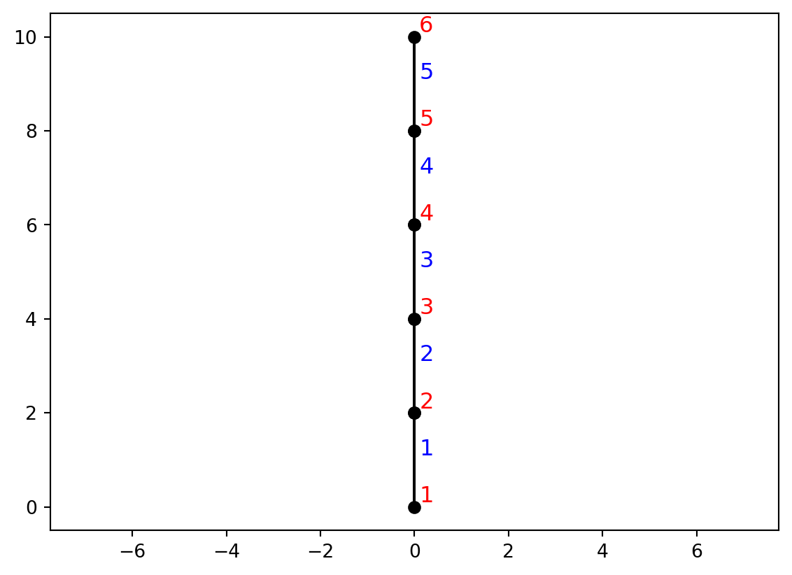
10.5 Eigenvalue Analysis
The natural frequency for a single-DOF problem, given in Equation 10.3, is derived for free undamped vibration. That version of the governing equations for multi-DOF problems reads
\[ \mathbf{M} \ddot{\mathbf{u}} + \mathbf{K}\mathbf{u} = \mathbf{0} \tag{10.8}\]
where \(\mathbf{M}=\) mass matrix and \(\ddot{\mathbf{u}}=\) acceleration along the DOFs of the structure. To solve that system of second-order differential equations we try the solution \(\mathbf{u}(t) = \boldsymbol{\upphi} \cdot \mathrm{sin}(\omega\cdot t)\). Substituting it into Equation 10.8 results in the generalized eigenvalue problem
\[ \left( \mathbf{K} - \omega^2 \mathbf{M} \right)\boldsymbol{\upphi}= \mathbf{0} \tag{10.9}\]
If we define \(\gamma \equiv \omega^2\) then \(\gamma\) is an eigenvalue and \(\boldsymbol{\upphi}\) is an eigenvector. The number of eigenvalues and eigenvectors equals the number of DOFs with mass. It is the lowest eigenvalues, i.e., the lowest natural frequencies that matter most in practice because higher modes take more energy to excite. The following function takes the stiffness and mass matrices in the Final DOF configuration and determines the eigenvalues and eigenvectors, sorting them from low to high frequency:
def eigenAnalysis(Kf, Mf):
    from scipy.linalg import eig
    allEigenInformation = eig(Kf, Mf, left=True, right=False)
    allEigenvalues = allEigenInformation[0]
    sortedEigenvalueIndices = np.argsort(np.abs(allEigenvalues))
    eigenvalues = []
    eigenvectors = []
    for i in range(len(sortedEigenvalueIndices)):
        if allEigenvalues[sortedEigenvalueIndices[i]].real == np.inf:
            pass
        else:
            eigenvalues.append(allEigenvalues[sortedEigenvalueIndices[i]].real)
            eigenvectors.append(allEigenInformation[1][:,sortedEigenvalueIndices[i]])
    for i in range(len(eigenvalues)):
        norm = np.linalg.norm(eigenvectors[i])
        eigenvectors[i] = eigenvectors[i] / norm
    numEigenvalues = len(eigenvalues)
    naturalFrequencies = []
    for i in range(numEigenvalues):
        frequency = np.sqrt(eigenvalues[i])
        naturalFrequencies.append(frequency)
    return eigenvalues, naturalFrequencies, eigenvectors
That function is utilized here to introduce a new function in the structural model class:
class model(model):
    def getNaturalFrequencies(self):
        ndof, ntot, F, Ma, elemlist = self.getData()
        free = range(ndof)
        ua = np.zeros((ntot,3))
        Ka = np.zeros((ntot, ntot))
        Ka = np.zeros((ntot, ntot))
        for i in range(len(elemlist)):
            id, xyz, ug = self.localize(i, ua)
            element = elemlist[i]
            element.initialize(xyz)
            Fg_tilde, Kg = element.stateDetermination(xyz, ug, 1.0)
            Ka[np.ix_(id, id)] = Ka[np.ix_(id,id)] + Kg
        Mf = Ma[np.ix_(free, free)]
        Kf = Ka[np.ix_(free, free)]
        gammas, omegas, phi = eigenAnalysis(Kf, Mf)
        print(f"Found {len(omegas)} natural frequencies:")
        for i in range(len(omegas)):
            Tn = 2*np.pi/omegas[i]
            print(f"Natural frequency number {i+1} is {omegas[i]:.1f} rad/sec. (period={Tn:.4f} sec.)")
        return omegas, phi
In turn, that function is now employed to conduct an eigenvalue analysis for the cantilevered column. The structural model must be created, to make it aware of the new function added to the model class:
structuralModel = model(input)
gammas, phi = structuralModel.getNaturalFrequencies()
Found 5 natural frequencies:
Natural frequency number 1 is 27.3 rad/sec. (period=0.2298 sec.)
Natural frequency number 2 is 164.2 rad/sec. (period=0.0383 sec.)
Natural frequency number 3 is 443.1 rad/sec. (period=0.0142 sec.)
Natural frequency number 4 is 827.0 rad/sec. (period=0.0076 sec.)
Natural frequency number 5 is 1211.6 rad/sec. (period=0.0052 sec.)nel number of natural frequencies are detected because that is the number of lumped masses specified in Listing 10.1. The eigenvectors are not printed here; they give the displaced shape of the structure for each natural frequency. For reference, the analytical solution for the first natural frequency of a cantilevered column with distributed mass is
\[ \omega_n \approx 1.875^2 \sqrt{\frac{EI}{\rho A \cdot L^4}} \tag{10.10}\]
Evaluating that formula gives
L = 10
omega_cantilever = 1.875**2 * np.sqrt(E*I/(rho*A*L**4))
print(f"Analytical first natural frequency: {omega_cantilever:.1f} rad/sec.")
Analytical first natural frequency: 27.8 rad/sec.which is close to the first natural frequency printed from Listing 10.4. That is expected; the more elements the cantilevered column is discretized into, the closer the first mode will be to the exact solution with distributed mass.
10.6 Modal Analysis
While not applied in this book, knowledge of modal analysis is helpful for subsequent derivations. The technique also provides insight into how a structure responds to dynamic load in distinct modes. Simply put, each mode is the displaced shape given by the eigenvector. In modal analysis, the total displacement of the structure is expressed as the modal expansion
\[ \mathbf{u}(t) = \sum_{n=1}^{N} \boldsymbol{\upphi}_n \cdot q_n(t) \tag{10.11}\]
where \(q_n(t)\) is a generalized DOF that determines the temporal variation of the displacement in mode number \(n\). Next, we collect all eigenvectors into the matrix \(\boldsymbol{\Phi} = [\boldsymbol{\upphi}_1 \;\boldsymbol{\upphi}_2 \; \cdots \;\boldsymbol{\upphi}_N \;]\) so that \(\mathbf{u}(t)=\boldsymbol{\Phi} \mathbf{q}(t)\), where \(\mathbf{q}(t)\) is a vector of all generalized DOFs from Equation 10.11. Substitution into Equation 10.8 gives
\[ \mathbf{M} \boldsymbol{\Phi} \ddot{\mathbf{q}} + \mathbf{K} \boldsymbol{\Phi} \mathbf{q} = \mathbf{0} \tag{10.12}\]
Premultiplying Equation 10.12 by \(\boldsymbol{\Phi}^{\top}\) gives
\[ \left[ \boldsymbol{\Phi}^{\top}\mathbf{M} \boldsymbol{\Phi}\right] \ddot{\mathbf{q}} + \left[\boldsymbol{\Phi}^{\top}\mathbf{K} \boldsymbol{\Phi} \right] \mathbf{q} = \mathbf{0} \tag{10.13}\]
It turns out that the two matrices marked with square brackets are diagonal matrices. The implication is that the system of equations in Equation 10.13 actually is \(N\) decoupled single-DOF problems on the form \(M_n \cdot \ddot{q}_n + K_n \cdot q_n=0\), where \(M_n=\boldsymbol{\upphi}_n^{\top} \mathbf{M}\boldsymbol{\upphi}_n=\) modal mass and \(K_n=\boldsymbol{\upphi}_n^{\top} \mathbf{K}\boldsymbol{\upphi}_n=\) modal stiffness. This decoupling of the multi-DOF system in Equation 10.8 is the essence of modal analysis. The modal load is the dot product \(F_n=\boldsymbol{\upphi}_n^{\top} \mathbf{F}\). Certain damping models, addressed next, supports the decoupling seen here.
10.7 Damping Models
Although hysteretic materials that take displacement as input is a source of energy dissipation, damping here means velocity-dependent force. In most structures, such as buildings and bridges, the damping is low. That statement is quantified for single-DOF problems by comparing \(C\) to the “critical damping” value,
\[ C_{cr} = 2\cdot M \cdot \omega_n = 2\cdot \sqrt{K\cdot M} \tag{10.14}\]
which is determined by solving the differential equation in Equation 10.1 with all three terms present on the left-hand side and zero loading on the right-hand side. A damping value \(C<C_{cr}\) is referred to as under-critical damping. That situation means the structure will oscillate, with steadily diminishing displacement amplitude, after the dynamic loading is over. In fact, \(C \ll C_{cr}\) for most structures and engineers typically specify damping via the ratio \(\zeta = \frac{C}{C_{cr}}\), obtaining \(C\) indirectly as
\[ C = \zeta \cdot C_{cr} = 2 \cdot \zeta \cdot M \cdot \omega_n = 2 \cdot \zeta \cdot \sqrt{K\cdot M} \tag{10.15}\]
For multi-DOF structures, damping is introduced via a damping matrix, \(\mathbf{C}\), which multiplies the vector of velocities along the DOFs, \(\dot{\mathbf{u}}\), shown here in the complete linear multi-DOF equations of motion:
\[ \mathbf{M} \ddot{\mathbf{u}}(t) + \mathbf{C} \ddot{\mathbf{u}}(t) + \mathbf{K}\mathbf{u}(t) = \mathbf{F}(t) \tag{10.16}\]
The matrix \(\mathbf{C}\) is artificial in the sense that it is not derived from physics. In fact, in linear analysis the aim is often to define a \(\mathbf{C}\) matrix that facilitates the modal decoupling described in the previous section. Such damping matrices are called classical, and the two most popular damping models have that characteristic. One of those options follows directly from Equation 10.15, referred to as modal damping. Specifically, if the damping \(C_n = 2 \zeta_n M_n \omega_n\) is applied to each mode, then the damping matrix implied by that is
\[ \mathbf{C} = \mathbf{M} \left( \sum_{n=1}^{N} \frac{2 \zeta_n \omega_n}{M_n} \boldsymbol{\upphi}_n \boldsymbol{\upphi}_n^{\top} \right) \mathbf{M} \tag{10.17}\]
This damping model is versatile, because it allows the specification of any damping at any mode. However, the modal damping matrix in Equation 10.17 is a full matrix, contrasting with \(\mathbf{M}\) and \(\mathbf{K}\), which are usually sparse and/or banded matrices. This is an important consideration for the equation solver that is utilized at every time increment.
The other popular damping model is called Rayleigh damping. It specifies \(\mathbf{C}\) by adding portions of \(\mathbf{K}\) and \(\mathbf{M}\):
\[ \mathbf{C} = c_M \cdot \mathbf{M} + c_K \cdot \mathbf{K} \tag{10.18}\]
where \(c_M\) and \(c_K\) are constants, determined next. Adopting the mantra of modal analysis, Equation 10.18 is pre- and post-multiplied by the eigenvector \(\boldsymbol{\upphi}_n\):
\[ C_n = \boldsymbol{\upphi}_n^{\top}\mathbf{C}\boldsymbol{\upphi}_n = c_M \cdot \boldsymbol{\upphi}_n^{\top}\mathbf{M}\boldsymbol{\upphi}_n + c_K \cdot \boldsymbol{\upphi}_n^{\top}\mathbf{K}\boldsymbol{\upphi}_n = c_M \cdot M_n + c_K \cdot K_n \tag{10.19}\]
Next, the modal damping, \(C_n\), is expressed as a fraction of the critical damping, as was done for single-DOF problems in Equation 10.14. Substitution of Equation 10.14, with subscripts \(n\) on both \(\zeta\) and \(M\), into Equation 10.19 gives
\[ \zeta_n = c_M \cdot \frac{1}{2 \omega_n} + c_K \cdot \frac{\omega_n}{2} \tag{10.20}\]
That equation is employed at two different frequencies, often the two first natural frequencies, \(\omega_1\) and \(\omega_2\), to solve for the two unknowns \(c_M\) and \(c_K\). That gives the damping ratio \(\zeta_1\) and \(\zeta_2\) at those two frequencies, respectively. If the same damping is specified at both frequencies, the expressions for the Rayleigh damping proportionality constants are
\[ c_M = \zeta \cdot \frac{2 \omega_1 \omega_2}{\omega_1+\omega_2} \tag{10.21}\]
and
\[ c_K = \zeta \cdot \frac{2}{\omega_1+\omega_2} \tag{10.22}\]
The damping at other frequencies is given by Equation 10.20, implying that the damping at other frequencies can be significantly different from the target damping. In summary, two damping models are considered in this chapter:
- Modal damping, defined by Equation 10.17, with identical target damping ratio, \(\zeta\), at all natural frequencies
- Rayleigh damping, defined by Equation 10.18, with identical target damping ratio, \(\zeta\), at the first two natural frequencies, with proportionality coefficients determined by Equation 10.21 and Equation 10.22
10.8 Damping Derivatives
For the response sensitivities derived and implemented later in this chapter, it is necessary to have the derivative of the damping matrix with respect to a generic variable, \(x\). Two scenarios are possible; the first and simplest is that \(x\) is the target damping ratio, \(\zeta\). In that case, the derivative of the modal damping matrix is
\[ \frac{\partial \mathbf{C}}{\partial x} = \mathbf{M} \left( \sum_{n=1}^{N} \frac{2 \omega_n}{M_n} \boldsymbol{\upphi}_n \boldsymbol{\upphi}_n^{\top} \right) \mathbf{M} \tag{10.23}\]
and the derivative of of the Rayleigh damping matrix is
\[ \frac{\partial \mathbf{C}}{\partial x} = \frac{\partial c_M}{\partial x} \cdot \mathbf{M} + \frac{\partial c_K}{\partial x} \cdot \mathbf{K} \tag{10.24}\]
with Equation 10.21 and Equation 10.22 giving
\[ \frac{\partial c_M}{\partial x} = \frac{2 \omega_1 \omega_2}{\omega_1+\omega_2} \tag{10.25}\]
and
\[ \frac{\partial c_K}{\partial x} = \frac{2}{\omega_1+\omega_2} \tag{10.26}\]
The other scenario is that \(x\) is a variable that affects the mass or stiffness matrices. In that case, the derivative of the modal damping matrix in Equation 10.17 is obtained with the product rule of differentiation:
\[ \begin{aligned} \frac{\partial \mathbf{C}}{\partial x} &= \frac{\partial \mathbf{M}}{\partial x} \left( \sum_{n=1}^{N} \frac{2 \zeta_n \omega_n}{M_n} \boldsymbol{\upphi}_n \boldsymbol{\upphi}_n^{\top} \right) \mathbf{M} \\ &+ \mathbf{M} \left( \sum_{n=1}^{N} \frac{2 \zeta_n }{M_n} \frac{\partial \omega_n}{\partial x} \boldsymbol{\upphi}_n \boldsymbol{\upphi}_n^{\top} \right) \mathbf{M} \\ &- \mathbf{M} \left( \sum_{n=1}^{N} \frac{2 \zeta_n \omega_n}{M_n^2} \frac{\partial M_n}{\partial x}\boldsymbol{\upphi}_n \boldsymbol{\upphi}_n^{\top} \right) \mathbf{M} \\ &+ \mathbf{M} \left( \sum_{n=1}^{N} \frac{2 \zeta_n \omega_n}{M_n} \frac{\partial \boldsymbol{\upphi}_n}{\partial x} \boldsymbol{\upphi}_n^{\top} \right) \mathbf{M} \\ &+ \mathbf{M} \left( \sum_{n=1}^{N} \frac{2 \zeta_n \omega_n}{M_n} \boldsymbol{\upphi}_n \frac{\partial \boldsymbol{\upphi}_n^{\top}}{\partial x} \right) \mathbf{M} \\ &+ \mathbf{M} \left( \sum_{n=1}^{N} \frac{2 \zeta_n \omega_n}{M_n} \boldsymbol{\upphi}_n \boldsymbol{\upphi}_n^{\top} \right) \frac{\partial \mathbf{M}}{\partial x} \\ \end{aligned} \tag{10.27}\]
That shows the need for the eigenvalue and eigenvector derivatives \(\frac{\partial \omega_n}{\partial x}\) and \(\frac{\boldsymbol{\upphi}_n}{\partial x}\). That is also the case for the derivative of the Rayleigh damping matrix, which now reads
\[ \frac{\partial \mathbf{C}}{\partial x} = \frac{\partial c_M}{\partial x} \cdot \mathbf{M} + c_M \cdot \frac{\partial \mathbf{M}}{\partial x} + \frac{\partial c_K}{\partial x} \cdot \mathbf{K} + c_K \cdot \frac{\partial \mathbf{K}}{\partial x} \tag{10.28}\]
with the derivative of Equation 10.21 now a bit more complex:
\[ \frac{\partial c_M}{\partial x} = \frac{\partial \omega_1}{\partial x} \cdot \frac{2 \zeta \omega_2}{\omega_1+\omega_2} + \frac{\partial \omega_2}{\partial x} \cdot \frac{2 \zeta \omega_1}{\omega_1+\omega_2} - \frac{2 \zeta \omega_1 \omega_2}{(\omega_1+\omega_2)^2} \left(\frac{\partial \omega_1}{\partial x} +\frac{\partial \omega_2}{\partial x} \right) \tag{10.29}\]
Similarly, the derivative of Equation 10.22 is
\[ \frac{\partial c_K}{\partial x} = - \frac{2 \zeta}{(\omega_1+\omega_2)^2} \left(\frac{\partial \omega_1}{\partial x} +\frac{\partial \omega_2}{\partial x} \right) \tag{10.30}\]
The need for eigenvalue and eigenvector derivatives is addressed next.
10.9 Eigen Derivatives
Consider the eigenvalue problem in Equation 10.9 written in index notation:
\[ \left( K_{ij} - \gamma M_{ij} \right) \phi_j = 0_i \tag{10.31}\]
The notation \(\gamma \equiv \omega^2\) means that \(\partial \omega / \partial x = (\partial \gamma / \partial x) / (2 \omega)\). To calculate the derivative of \(\gamma\) it is necessary to impose a rule that normalizes the eigenvectors. The criterion \(||\boldsymbol{\upphi}|| \equiv \sqrt{\phi_m \phi_m} = 1\) is employed here, i.e., scaling the eigenvectors to unit length. The result of that, needed shortly, is
\[ \begin{aligned} \frac{\partial ||\boldsymbol{\upphi}||}{\partial x} &= \frac{1}{2} \cdot \frac{1}{\sqrt{\phi_m \phi_m}} \cdot \frac{\partial \left(\phi_m \phi_m \right)}{\partial x} \\ &= \frac{1}{2} \cdot \frac{1}{\sqrt{\phi_m \phi_m}} \cdot 2 \cdot \phi_m \frac{\partial \phi_m}{\partial x} \\ &= \boldsymbol{\upphi}^\text{T} \frac{\partial \boldsymbol{\upphi}}{\partial x} = 0 \end{aligned} \tag{10.32}\]
Differentiation of Equation 10.31 with respect to \(x\) gives
\[ \frac{\partial K_{ij}}{\partial x} \phi_j - \frac{\partial \gamma}{\partial x} M_{ij} \phi_j - \gamma \frac{\partial M_{ij}}{\partial x} \phi_j + \left( K_{ij} - \gamma M_{ij} \right) \frac{\partial \phi_j}{\partial x} = 0_i \tag{10.33}\]
Multiplying through by \(\phi_i\) yields
\[ \phi_i \frac{\partial K_{ij}}{\partial x} \phi_j - \phi_i \frac{\partial \gamma}{\partial x} M_{ij} \phi_j - \phi_i \gamma \frac{\partial M_{ij}}{\partial x} \phi_j + \phi_i \left( K_{ij} - \gamma M_{ij} \right) \frac{\partial \phi_j}{\partial x} = 0 \tag{10.34}\]
Because \(\left( K_{ij} - \gamma M_{ij} \right)\) is symmetric, it is possible to interchange \(i\) and \(j\) in that parenthesis, meaning that the product \(\phi_i \left( K_{ij} - \gamma M_{ij} \right)\) can be written \(\left( \mathbf{K} - \gamma \mathbf{M} \right) \boldsymbol{\upphi}^\text{T}\) in vector-matrix notation. As a result, the last term in Equation 10.34 is written \(\left( \mathbf{K} - \gamma \mathbf{M} \right) \boldsymbol{\upphi}^\text{T} \frac{\partial \boldsymbol{\upphi}}{\partial x}\). In turn, that leads the last term in Equation 10.34 to vanish because Equation 10.32 shows that \(\boldsymbol{\upphi}^\text{T} \frac{\partial \boldsymbol{\upphi}}{\partial x}\) is zero. Solving Equation 10.34 for \(\partial \gamma / \partial x\) gives the following result:
\[ \frac{\partial \gamma}{\partial x} = \frac{\phi_i \frac{\partial K_{ij}}{\partial x} \phi_j - \gamma \phi_i \frac{\partial M_{ij}}{\partial x} \phi_j}{\phi_i M_{ij} \phi_j } \tag{10.35}\]
Equation 10.33 is revisited in order to determine the associated eigenvector derivative. The matrix \(\left( K_{ij} - \gamma M_{ij} \right)\) is singular, but a solution is obtained by calculating its pseudo-inverse, which yields
\[ \frac{\partial \phi_j}{\partial x} = \left( K_{ij} - \gamma M_{ij} \right)^+ \left( -\frac{\partial K_{ij}}{\partial x} + \frac{\partial \gamma}{\partial x} M_{ij} + \gamma \frac{\partial M_{ij}}{\partial x} \right) \phi_j \tag{10.36}\]
The following function takes input from Listing 10.3 and calculates the eigenvalue and eigenvector derivatives derived above:
def eigenDerivatives(Kf, dKf, Mf, dMf, eigenvalues, eigenvectors):
    dgammas = []
    domegas = []
    dvectors = []
    for i in range(len(eigenvalues)):
        lhs = (eigenvectors[i].dot(Mf)).dot(eigenvectors[i])
        rhs = (eigenvectors[i].dot(dKf)).dot(eigenvectors[i]) - \
                eigenvalues[i] * (eigenvectors[i].dot(dMf)).dot(eigenvectors[i])
        dgammas.append(rhs/lhs)
        domegas.append(0.5 / np.sqrt(eigenvalues[i]) * rhs/lhs)
        coefficientMatrix = np.subtract(Kf, np.multiply(eigenvalues[i], Mf))
        rhsParenthesis = np.multiply(dgammas[i], Mf) + np.multiply(eigenvalues[i], dMf) - dKf
        dvectors.append(np.linalg.pinv(coefficientMatrix).dot(rhsParenthesis).dot(eigenvectors[i]))
    return dgammas, domegas, dvectors
10.10 Load from Ground Motion
Earthquake ground motion is specified as time-varying acceleration of the ground. Usually, it is horizontal ground motion that is causing damage to structures. Therefore, in this book, uni-directional horizontal ground motion is considered. Such ground motions can be downloaded from online databases or they can be generated as shown in Chapter 13. Appendix C contains the famous El Centro ground motion from a magnitude 6.9 earthquake that occurred in Imperial Valley in Southern California on May 18, 1940. The following function is developed to read such ground motions from a file:
def readGroundMotion(fileName, dt, percentPadding=0.0):
    file = open(fileName, "r")
    lines = file.readlines()
    splitline = lines[0].split()
    if splitline[0].isalpha():
        del lines[:4]
    t = [0.0]
    rawGroundMotion = [0.0]
    for oneline in lines:
        splitline = oneline.split()
        for j in range(len(splitline)):
            value = 9.81 * float(splitline[j])
            t.append(t[-1]+dt)
            rawGroundMotion.append(value)
    for i in range(int(percentPadding/100*len(rawGroundMotion))):
        t.append(t[-1]+dt)
        rawGroundMotion.append(0.0)
    metersPerSec2GroundMotionMatrix = np.concatenate(([t], [rawGroundMotion]), axis=0)
    return metersPerSec2GroundMotionMatrix
The following remarks are attached to that function:
- It is assumed that the ground acceleration values in the file are in the unit of \(g\)
- The output of the function is in the unit of metres per second squared
- The function takes \(dt\) as input; the user must carefully check that the correct value is provided; typical values are 0.005, 0.01, and 0.02 seconds
- If letters are found in the first line of the file then the first four lines are removed, thus adopting a common ground motion database protocol
- The function returns one matrix with two columns: the time axis and the corresponding acceleration values
Here is a plot of the El Centro ground motion, read from a file named ElCentro.txt, created by saving the content of Appendix C:
dt = 0.02
gmMatrix = readGroundMotion("ElCentro.txt", dt)
plt.figure()
plt.plot(gmMatrix[0], gmMatrix[1], 'k-', linewidth=1.0)
plt.xlabel("Time [sec.]")
plt.ylabel("Ground Acceleration [$\\frac{m}{s^2}$]")
plt.grid(True)
plt.show()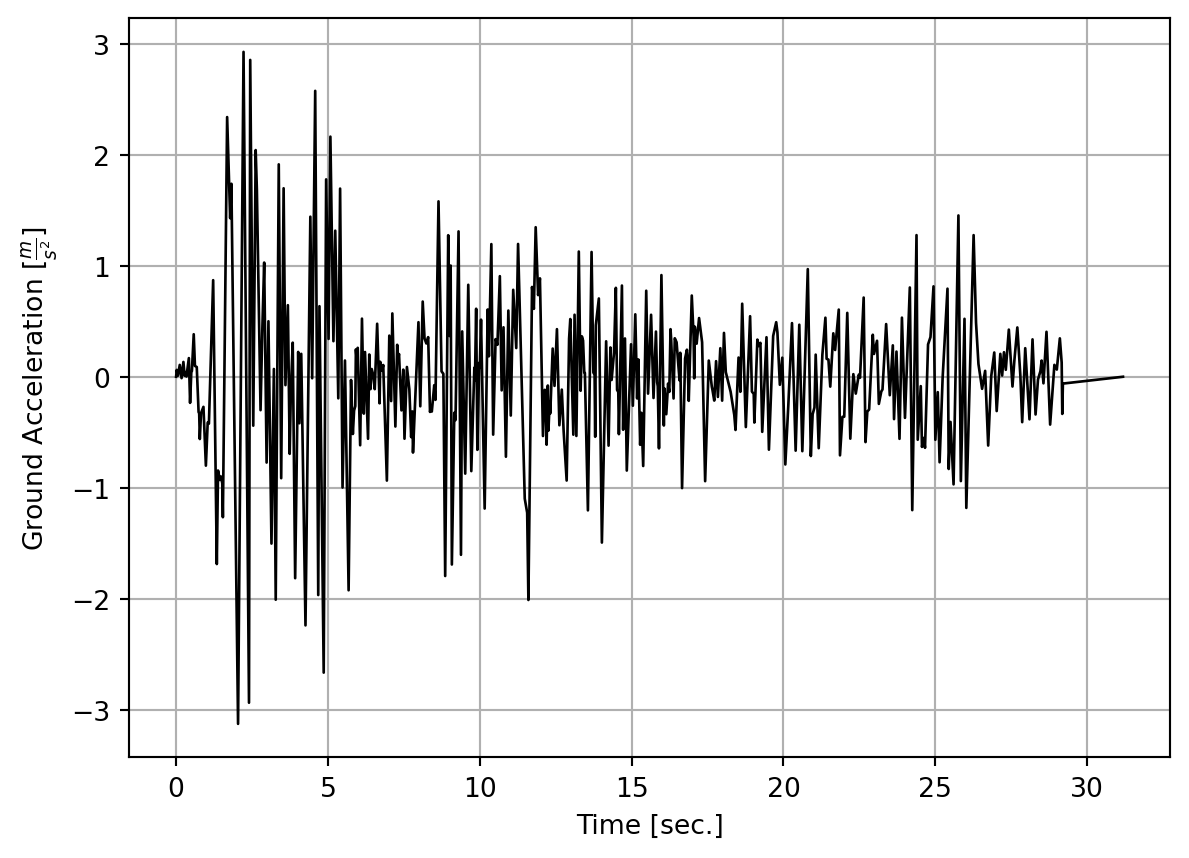
If lumped structural mass is specified solely for horizontal DOFs, then the load vector is a simple extension of the right-hand side of Equation 10.1:
\[ \mathbf{F}(t) = - \mathbf{M} \cdot \ddot{u}_g(t) \tag{10.37}\]
If mass is specified along DOFs in other directions than the ground motion, or if the ground motion is multi-directional, then a selection vector is introduced in Equation 10.37 to multiply the ground acceleration with the correct masses.
10.11 Time-stepping Scheme
The governing equilibrium equations for linear multi-DOF problems are given in Equation 10.16. To solve them computationally for arbitrary loading, the time axis is discretized into increments. The governing equations at time \(t_{n+1}\) are written
\[ \mathbf{M} \ddot{\mathbf{u}}_{n+1} + \mathbf{C} \ddot{\mathbf{u}}_{n+1} + \mathbf{K}\mathbf{u}_{n+1} = \mathbf{F}_{n+1} \tag{10.38}\]
where the symbol \(n\) that appears here is unrelated to the subscript of \(\omega_n\) and \(\boldsymbol{\upphi}_n\) see earlier. Many time-stepping schemes to solve Equation 10.38 are available. Most of them employ the solution at increment \(t_n\) to obtain the solution at \(t_{n+1}\). Such methods can be generically written
\[ \begin{aligned} \ddot{\mathbf{u}}_{n+1} &= a_1 \cdot \mathbf{u}_{n+1} + a_2 \cdot \mathbf{u}_n + a_3 \cdot \dot{\mathbf{u}}_n + a_4 \cdot \ddot{\mathbf{u}}_n \\ \dot{\mathbf{u}}_{n+1} &= a_5 \cdot \mathbf{u}_{n+1} + a_6 \cdot \mathbf{u}_n + a_7 \cdot \dot{\mathbf{u}}_n + a_8 \cdot \ddot{\mathbf{u}}_n \end{aligned} \tag{10.39}\]
A popular choice for the constants is \(a_1=\frac{4}{\Delta t^2}\), \(a_2=-a_1\), \(a_3=-\frac{4}{\Delta t}\), \(a_4=-1\), \(a_5=\frac{2}{\Delta t}\), \(a_6=-a_5\), \(a_7=-1\), and \(a_8=0\). That means the Newmark-beta method with \(\beta=0.25\) and \(\gamma=0.5\), corresponding to the constant average acceleration method. Substitution of Equation 10.39 into Equation 10.16 and rearranging gives the following system of equations:
\[ \begin{aligned} \left(a_1 \mathbf{M} + a_5 \mathbf{C} + \mathbf{K} \right) \mathbf{u}_{n+1} &= \mathbf{F}_{n+1} \\ &- \left(a_4 \mathbf{M} + a_8 \mathbf{C} \right) \ddot{\mathbf{u}}_n \\ &- \left(a_3 \mathbf{M} + a_7 \mathbf{C} \right) \dot{\mathbf{u}}_n \\ &- \left(a_2 \mathbf{M} + a_6 \mathbf{C} \right) \mathbf{u}_n \end{aligned} \tag{10.40}\]
Equation 10.40 is an expanded version of the linear static case \(\mathbf{K}\mathbf{u}=\mathbf{F}\). That is why the parenthesis in the left-hand side is called the effective dynamic stiffness. Equation 10.40 is solved in the analysis algorithm presented later in this chapter, after the differentiation of Equation 10.38.
10.12 First-order Sensitivities
Applying the product rule of differentiation to Equation 10.38 yields
\[ \begin{aligned} &\phantom{=}\frac{\partial \mathbf{M}}{\partial x} \ddot{\mathbf{u}}_{n+1} + \mathbf{M} \frac{\partial \ddot{\mathbf{u}}_{n+1}}{\partial x} \\ &+ \frac{\partial \mathbf{C}}{\partial x} \ddot{\mathbf{u}}_{n+1} + \mathbf{C} \frac{\partial \ddot{\mathbf{u}}_{n+1}}{\partial x} \\ &+ \frac{\partial \mathbf{K}}{\partial x}\mathbf{u}_{n+1} + \mathbf{K}\frac{\partial \mathbf{u}_{n+1}}{\partial x} \\ &= \frac{\partial \mathbf{F}_{n+1}}{\partial x} \end{aligned} \tag{10.41}\]
Substitution of Equation 10.39 and rearranging gives a linear system of equations with the same coefficient matrix as Equation 10.40:
\[ \begin{aligned} \left(a_1 \mathbf{M} + a_5 \mathbf{C} + \mathbf{K} \right) \frac{\partial \mathbf{u}_{n+1}}{\partial x} &= \frac{\partial \mathbf{F}_{n+1}}{\partial x} \\ &- \frac{\partial \mathbf{M}}{\partial x} \left(a_1 \mathbf{u}_{n+1} + a_2 \mathbf{u}_n + a_3 \dot{\mathbf{u}}_n + a_4 \ddot{\mathbf{u}}_n \right) \\ &- \mathbf{M} \left(a_2 \frac{\partial \mathbf{u}_n}{\partial x} + a_3 \frac{\partial \dot{\mathbf{u}}_n}{\partial x} + a_4 \frac{\partial \ddot{\mathbf{u}}_n}{\partial x} \right) \\ &- \frac{\partial \mathbf{C}}{\partial x} \left(a_5 \mathbf{u}_{n+1} + a_6 \mathbf{u}_n + a_7 \dot{\mathbf{u}}_n + a_8 \ddot{\mathbf{u}}_n \right) \\ &- \mathbf{C} \left(a_6 \frac{\partial \mathbf{u}_n}{\partial x} + a_7 \frac{\partial \dot{\mathbf{u}}_n}{\partial x} + a_8 \frac{\partial \ddot{\mathbf{u}}_n}{\partial x} \right) \\ &- \frac{\partial \mathbf{K}}{\partial x} \mathbf{u}_{n+1} \end{aligned} \tag{10.42}\]
Notice that the response \(\mathbf{u}_{n+1}\) appears in the right-hand side, meaning it must be determined before solving for response sensitivities. Equation 10.40 and Equation 10.42 are solved sequentially in the algorithm provided in the next section.
10.13 Analysis Algorithm
Putting together the derivations made in this chapter, the following algorithm calculates the linear dynamic response of multi-DOF structures, together with first-order response sensitivities:
def linearDynamicAnalysis(structuralModel, dampingModel, dampingRatio, groundMotion, trackNode, trackDOF, DDMparameters=[]):
    from scipy.linalg import lu_factor, lu_solve

    # Ground motion
    t = groundMotion[0]
    dt = float(t[1] - t[0])
    groundAcceleration = groundMotion[1]

    # Mass matrix
    ndof, ntot, F, Ma, elemlist = structuralModel.getData()
    free = range(ndof)
    nelem = len(elemlist)
    Mf = Ma[np.ix_(free, free)]

    # Stiffness matrix
    ua = np.zeros((ntot,3))
    Ka = np.zeros((ntot, ntot))
    for i in range(nelem):
        id, xyz, ug = structuralModel.localize(i, ua)
        element = elemlist[i]
        element.initialize(xyz)
        Fg_tilde, Kg = element.stateDetermination(xyz, ug, 1.0)
        Ka[np.ix_(id, id)] = Ka[np.ix_(id,id)] + Kg
    Kf = Ka[np.ix_(free, free)]

    # Damping matrix
    eigenvalues, naturalFrequencies, eigenvectors = eigenAnalysis(Kf, Mf)
    numEigenvalues = len(eigenvalues)
    if dampingModel == 'Rayleigh':
        omega1 = naturalFrequencies[0]
        omega2 = naturalFrequencies[1]
        factor = 2 * dampingRatio / (omega1 + omega2)
        cM = omega1 * omega2 * factor
        cK = factor
        Cf = np.multiply(Mf, cM) + np.multiply(Kf, cK)
    elif dampingModel == 'Modal':
        Sum = np.zeros((len(free), len(free)))
        for i in range(numEigenvalues):
            modalMass = (eigenvectors[i].dot(Mf)).dot(eigenvectors[i])
            outerProduct = np.outer(eigenvectors[i], eigenvectors[i])
            Sum += 2.0 * dampingRatio * np.sqrt(eigenvalues[i]) / modalMass * outerProduct
        Cf = (Mf.dot(Sum)).dot(Mf)

    # Initialization
    displacementOld = np.zeros(ndof)
    velocityOld = np.zeros(ndof)
    accelerationOld = np.zeros(ndof)
    ddmDisplacementOld = np.zeros((ndof, len(DDMparameters)))
    ddmVelocityOld = np.zeros((ndof, len(DDMparameters)))
    ddmAccelerationOld = np.zeros((ndof, len(DDMparameters)))
    ddmua = np.zeros(ntot)

    # Prepare for time-stepping
    a1=4/dt**2; a2=-a1; a3=-4/dt; a4=-1; a5=2/dt; a6=-a5; a7=-1; a8=0
    newDispFactor = np.multiply(a1, Mf) + np.multiply(a5, Cf)
    Keffective = newDispFactor + Kf
    dispFactor = np.multiply(a2, Mf) + np.multiply(a6, Cf)
    velocFactor = np.multiply(a3, Mf) + np.multiply(a7, Cf)
    accelFactor = np.multiply(a4, Mf) + np.multiply(a8, Cf)
    LU = lu_factor(Keffective)
    index = structuralModel.DOF[trackNode-1, trackDOF-1]
    trackDisp = []
    trackAllDDMs = np.zeros((len(DDMparameters), len(t)))

    # Loop over time increments
    for step in range(len(t)):
        Fnew = np.multiply(-np.diag(Mf), groundAcceleration[step])
        rhsNew = Fnew - dispFactor.dot(displacementOld) - velocFactor.dot(velocityOld) - accelFactor.dot(accelerationOld)
        displacementNew = lu_solve(LU, rhsNew)
        accelerationNew = np.multiply(a1, displacementNew) + np.multiply(a2, displacementOld) + np.multiply(a3, velocityOld) + np.multiply(a4, accelerationOld)
        velocityNew = np.multiply(a5, displacementNew) + np.multiply(a6, displacementOld) + np.multiply(a7, velocityOld) + np.multiply(a8, accelerationOld)
        trackDisp.append(displacementNew[index])

        # Sensitivity analysis
        if len(DDMparameters) > 0:
            ua[free, 0] = displacementNew
            for ddmIndex in range(len(DDMparameters)):
                theDampingRatioIsTheDDMparameter = False
                dKa = np.zeros((ntot, ntot))
                dMa = np.zeros((ntot, ntot))
                ddmRHSa = np.zeros(ntot)
                dcMdtheta = 0.0
                dcKdtheta = 0.0
                if DDMparameters[ddmIndex][0] == 'Element':
                    for eleNum in DDMparameters[ddmIndex][2]:
                        i = eleNum - 1
                        id, xyz, ug = structuralModel.localize(i, ua)
                        element = elemlist[i]
                        ddmRHSg, dKg, dKgdug = element.stateDerivative(xyz, ug, 1.0, DDMparameters[ddmIndex][1], 0, True)
                        ddmRHSa[id] = ddmRHSa[id] + ddmRHSg
                        dKa[np.ix_(id, id)] = dKa[np.ix_(id,id)] + dKg
                elif DDMparameters[ddmIndex][0] == 'Node' and DDMparameters[ddmIndex][1] == 'M':
                    dMa = structuralModel.getMassDerivative(DDMparameters[ddmIndex][2])
                    ddmRHSa = np.multiply(np.diag(dMa), groundAcceleration[step])
                elif DDMparameters[ddmIndex][0] == 'Model' and DDMparameters[ddmIndex][1] == 'targetDamping':
                    theDampingRatioIsTheDDMparameter = True
                dKf = dKa[np.ix_(free, free)]
                dMf = dMa[np.ix_(free, free)]
                dgammas, domegas, dvectors = eigenDerivatives(Kf, dKf, Mf, dMf, eigenvalues, eigenvectors)
                ddmRHSf = -ddmRHSa[free]
                ddmRHSf -= dispFactor.dot(ddmDisplacementOld[:,ddmIndex]) + velocFactor.dot(ddmVelocityOld[:,ddmIndex]) + accelFactor.dot(ddmAccelerationOld[:,ddmIndex])
                ddmRHSf -= dMf.dot(a1 * displacementNew + a2 * displacementOld + a3 * velocityOld + a4 * accelerationOld)
                a5parenthesis = a5 * displacementNew + a6 * displacementOld + a7 * velocityOld + a8 * accelerationOld

                if dampingModel == 'Rayleigh':
                    ddmRHSf -= cM * dMf.dot(a5parenthesis)
                    ddmRHSf -= cK * dKf.dot(a5parenthesis)
                    ddmRHSf -= dcMdtheta * Mf.dot(a5parenthesis)
                    ddmRHSf -= dcKdtheta * Kf.dot(a5parenthesis)
                    if theDampingRatioIsTheDDMparameter:
                        dfactor = 2 / (omega1 + omega2)
                        dcM = omega1 * omega2 * dfactor
                        dcK = dfactor
                    else:
                        domega1 = domegas[0]
                        domega2 = domegas[1]
                        dfactor = -2 * dampingRatio / (omega1 + omega2)**2 * (domega1 + domega2)
                        dcM = domega1 * omega2 * factor + omega1 * domega2 * factor + omega1 * omega2 * dfactor
                        dcK = dfactor
                    ddmRHSf -= dcM * Mf.dot(a5parenthesis)
                    ddmRHSf -= dcK * Kf.dot(a5parenthesis)

                elif dampingModel == 'Modal':
                    if theDampingRatioIsTheDDMparameter:
                        Sum = np.zeros((len(free), len(free)))
                        for i in range(numEigenvalues):
                            modalMass = (eigenvectors[i].dot(Mf)).dot(eigenvectors[i])
                            outerProduct = np.outer(eigenvectors[i], eigenvectors[i])
                            Sum += 2.0 * np.sqrt(eigenvalues[i]) / modalMass * outerProduct
                        dCf = (Mf.dot(Sum)).dot(Mf)
                    else:
                        term1 = np.zeros((len(free), len(free)))
                        term2 = np.zeros((len(free), len(free)))
                        term3 = np.zeros((len(free), len(free)))
                        term4 = np.zeros((len(free), len(free)))
                        term5 = np.zeros((len(free), len(free)))
                        term6 = np.zeros((len(free), len(free)))
                        for i in range(numEigenvalues):
                            modalMass = (eigenvectors[i].dot(Mf)).dot(eigenvectors[i])
                            dmodalmass = (dvectors[i].dot(Mf)).dot(eigenvectors[i]) + (eigenvectors[i].dot(dMf)).dot(eigenvectors[i]) + (eigenvectors[i].dot(Mf)).dot(dvectors[i])
                            outer1 = np.outer(eigenvectors[i], eigenvectors[i])
                            outer2 = np.outer(dvectors[i], eigenvectors[i])
                            outer3 = np.outer(eigenvectors[i], dvectors[i])
                            term1 = term1 + 2.0 * dampingRatio * np.sqrt(eigenvalues[i]) / modalMass * outer1
                            term2 = term2 + 2.0 * dampingRatio * 0.5 / np.sqrt(eigenvalues[i]) * dgammas[i] / modalMass * outer1
                            term3 = term3 + 2.0 * dampingRatio * np.sqrt(eigenvalues[i]) / modalMass**2 * dmodalmass * outer1
                            term4 = term4 + 2.0 * dampingRatio * np.sqrt(eigenvalues[i]) / modalMass * outer2
                            term5 = term5 + 2.0 * dampingRatio * np.sqrt(eigenvalues[i]) / modalMass * outer3
                            term6 = term6 + 2.0 * dampingRatio * np.sqrt(eigenvalues[i]) / modalMass * outer1
                        dCf = (dMf.dot(term1)).dot(Mf)
                        dCf += (Mf.dot(term2)).dot(Mf)
                        dCf -= (Mf.dot(term3)).dot(Mf)
                        dCf += (Mf.dot(term4)).dot(Mf)
                        dCf += (Mf.dot(term5)).dot(Mf)
                        dCf += (Mf.dot(term6)).dot(dMf)
                    ddmRHSf -= dCf.dot(a5parenthesis)

                ddmDisplacementNew = lu_solve(LU, ddmRHSf)
                ddmAccelerationNew = np.multiply(a1, ddmDisplacementNew) + np.multiply(a2, ddmDisplacementOld[:,ddmIndex]) + np.multiply(a3, ddmVelocityOld[:,ddmIndex]) + np.multiply(a4, ddmAccelerationOld[:,ddmIndex])
                ddmVelocityNew = np.multiply(a5, ddmDisplacementNew) + np.multiply(a6, ddmDisplacementOld[:,ddmIndex]) + np.multiply(a7, ddmVelocityOld[:,ddmIndex]) + np.multiply(a8, ddmAccelerationOld[:,ddmIndex])

                ddmDisplacementOld[:,ddmIndex] = ddmDisplacementNew
                ddmVelocityOld[:,ddmIndex] = ddmVelocityNew
                ddmAccelerationOld[:,ddmIndex] = ddmAccelerationNew

                ddmua[free] = ddmDisplacementNew
                trackAllDDMs[ddmIndex, step] = ddmua[index]
        displacementOld = displacementNew
        velocityOld = velocityNew
        accelerationOld = accelerationNew

    return trackDisp, trackAllDDMs
10.14 Column Example
The following analysis subjects the cantilevered column established in Section 10.4 to the El Centro ground motion. The following code says that the horizontal displacement at the top of the column is the response of interest. It also specifies that the three input variables for which response sensitivities are sought are stiffness, mass, and damping:
trackNode = nel+1
trackDOF = 1
dampingModel = 'Rayleigh'
dampingRatio = 0.05

# Derivative of mass matrix with respect to lumped mass
dM = [[0, 0, 0]]
for i in range(nel-1):
    dM.append([1, 0, 0])
dM.append([0.5, 0, 0])

# Sensitivity request
DDMparameters = [['Element', 'E', range(1, nel+1)],
                 ['Node', 'M', dM],
                 ['Model', 'targetDamping']]
The analysis is now run, with the displacement response plotted below:
u, dudx = linearDynamicAnalysis(structuralModel, dampingModel, dampingRatio, gmMatrix, trackNode, trackDOF, DDMparameters)
t = gmMatrix[0]
plt.figure()
plt.plot(t, u, 'k-', linewidth=1.0)
plt.xlabel("Time [sec.]")
plt.ylabel("Displacement [m]")
plt.grid(True)
plt.show()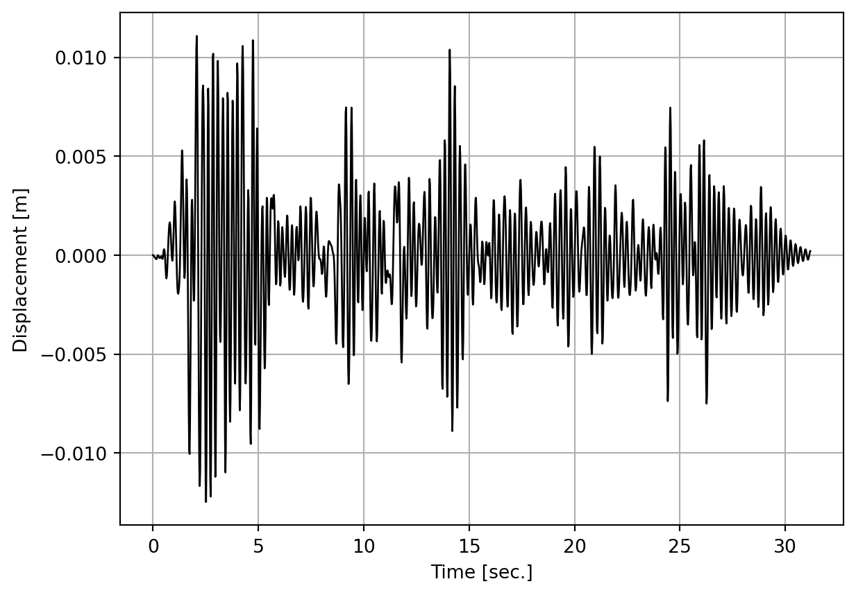
Next, the three response sensitivities are examined. They are made comparable by multiplying each \(\frac{\partial u}{\partial x}\) by the standard deviation of the respective variable, with a 10% coefficient of variation applied to all variables:
plt.figure()
plt.plot(t, dudx[0]*0.1*E, 'b-', linewidth=1.0, label='$\\frac{\\partial u}{\\partial E}$')
plt.plot(t, dudx[1]*0.1*A*L/nel*rho, 'm-', linewidth=1.0, label='$\\frac{\\partial u}{\\partial M}$')
plt.plot(t, dudx[2]*0.1*dampingRatio, 'c-', linewidth=1.0, label='$\\frac{\\partial u}{\\partial \\zeta}$')
plt.xlabel("Time [sec.]")
plt.ylabel("Displacement [m]")
plt.grid(True)
plt.legend(loc='upper right')
plt.show()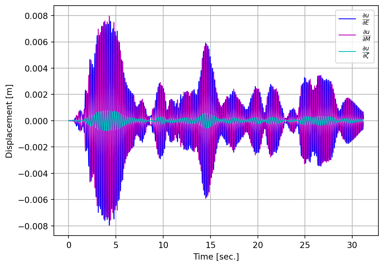
The response sensitivities presented in this book are verified by finite difference analysis in Chapter 14. The plot above suggests that stiffness and mass are far more important than the damping ratio, at least for a uniform 10% coefficient of variation. However, the plot is hard to read and a zoomed view is provided below:
timeWindow = range(int(0.12*len(t)), int(0.18*len(t)))
plt.figure()
plt.plot(t[timeWindow], np.array(u)[timeWindow], 'k-', linewidth=1.0, label='$u$')
plt.plot(t[timeWindow], dudx[0, timeWindow]*0.1*E, 'b-', linewidth=1.0, label='$\\frac{\\partial u}{\\partial E}$')
plt.plot(t[timeWindow], dudx[1, timeWindow]*0.1*A*L/nel*rho, 'm-', linewidth=1.0, label='$\\frac{\\partial u}{\\partial M}$')
plt.plot(t[timeWindow], dudx[2, timeWindow]*0.1*dampingRatio, 'c-', linewidth=1.0, label='$\\frac{\\partial u}{\\partial \\zeta}$')
plt.xlabel("Time [sec.]")
plt.grid(True)
plt.legend(loc='upper right')
plt.show()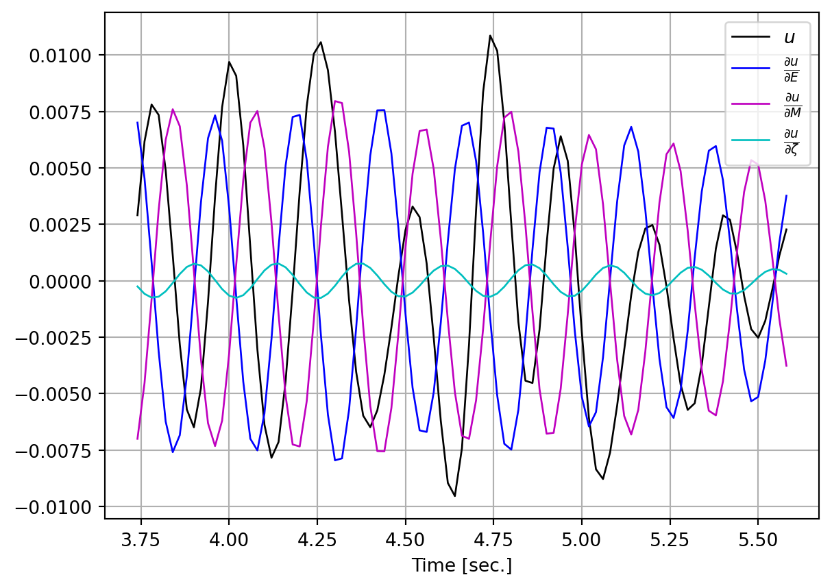
A pattern emerges when examining that plot. The stiffness and mass sensitivities are close to zero whenever the displacement peaks. That is not the case for the damping sensitivity. If it is the peak response that is of interest, as it usually is in earthquake engineering, the plot suggests that the peak response may not be as sensitive to mass and damping as first seemed the case.
To investigate, a plot of the quantity \(u+\sum_{i=1}^{3} \frac{\partial u}{\partial x_i} \sigma_i\) is created. That sum is over the quantities plotted in the previous figure. Below, that sum is accumulated one variable at a time. Moreover, the stiffness is increased while the mass and damping ratio are decreased. The cyan-coloured line is the final sum:
plt.figure()
plt.plot(t[timeWindow], np.array(u)[timeWindow], 'k-', linewidth=1.0, markersize=3, label='$u$')
term1 = np.array(u)[timeWindow] + dudx[0, timeWindow]*0.1*E
plt.plot(t[timeWindow], term1, 'b-', linewidth=1.0, label='E added')
term2 = term1 - dudx[1, timeWindow]*0.1*A*L/nel*rho
plt.plot(t[timeWindow], term2, 'm-', linewidth=1.0, label='E and M added')
term3 = term2 - dudx[2, timeWindow]*0.1*dampingRatio
plt.plot(t[timeWindow], term3, 'c-', linewidth=1.0, label='Damping also added')
plt.xlabel("Time [sec.]")
plt.grid(True)
plt.legend(loc='upper right')
plt.show()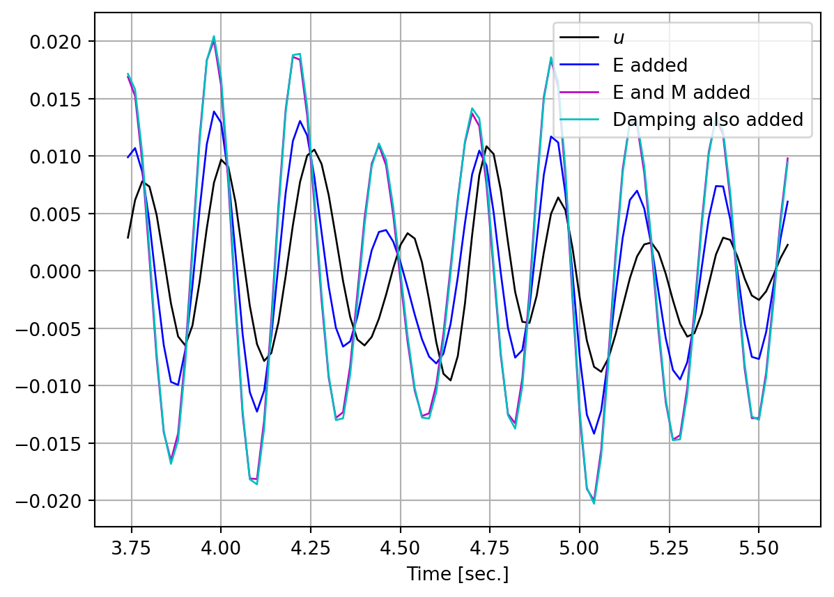
Here is the same plot, but now the stiffness is decreased while the mass and damping ratio are increased:
plt.figure()
plt.plot(t[timeWindow], np.array(u)[timeWindow], 'k-', linewidth=1.0, markersize=3, label='$u$')
term1 = np.array(u)[timeWindow] - dudx[0, timeWindow]*0.1*E
plt.plot(t[timeWindow], term1, 'b-', linewidth=1.0, label='E added')
term2 = term1 + dudx[1, timeWindow]*0.1*A*L/nel*rho
plt.plot(t[timeWindow], term2, 'm-', linewidth=1.0, label='E and M added')
term3 = term2 + dudx[2, timeWindow]*0.1*dampingRatio
plt.plot(t[timeWindow], term3, 'c-', linewidth=1.0, label='Damping also added')
plt.xlabel("Time [sec.]")
plt.grid(True)
plt.legend(loc='upper right')
plt.show()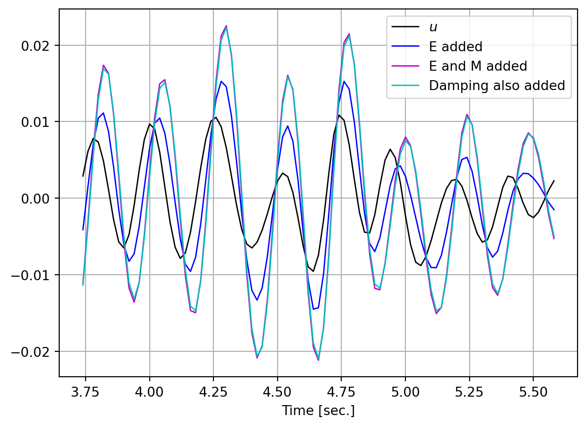
Both plots reveal that the peaks of the response both shift and grow when the stiffness and/or mass values change. Although the sensitivity is less than it first appeared, both plots confirm that damping is not highly influential, for the coefficient of variation considered here.